Mediator variables, sales funnel and frontdoor adjustment

Front-door adjustment on-the-fly

In Marketing Mix Modeling (MMM), we often encounter variables that sit between the marketing investment and the final conversion (sales). These are called mediators. Common examples include website visits, app installs, lead generation, or footfall in a store.

A common dilemma is whether to include these mediators in the MMM:

If we exclude them: We lose valuable information. Mediators are often measured more accurately or with higher frequency than sales, and they can help explain variance.
If we include them naively: We risk “blocking” the effect of the media. If the causal path is Media -> Visits -> Sales, and we control for Visits in a regression, the coefficient for Media will reflect only the direct effect of Media on Sales (which might be zero), not the total effect. This leads to underestimating the ROI of the media channel.

This tutorial demonstrates how to use Prophetverse to model this causal chain explicitly. We will build a model that respects the funnel structure: Investment drives Visits, and Visits drive Sales. This allows us to use the data from visits to improve our estimates without breaking the causal inference for investment ROI.

Data Generation

First, let’s generate some synthetic data where the ground truth is known. We assume a simple funnel:

Investment drives Visits (with adstock and saturation).
Visits drive Sales (with a conversion rate).
There is no direct path from Investment to Sales (Direct Effect = 0).
There is also some seasonality affecting both.

graph LR
    I[Investment] --> V[Visits]
    V --> S[Sales]
    Se[Seasonality] --> I
    Se --> S

Code

from prophetverse import (
    Prophetverse,
    Constant,
    LinearFourierSeasonality,
    GeometricAdstockEffect,
    MultiplyEffects,
    Forward,
    IgnoreInput,
    MichaelisMentenEffect,
    PriorPredictiveInferenceEngine,
    ChainedEffects,
)
from prophetverse.utils.regex import exact
import numpyro.distributions as dist
import numpy as np
import pandas as pd

# Synthetic data


rng = np.random.default_rng(42)
n = 356
idx = pd.period_range(start="2020-01-01", periods=n, freq="D")
X = pd.DataFrame(index=idx)
X["investment"] = rng.normal(loc=500, scale=100, size=n).clip(min=0)
X["investment"] += 100 * np.sin(np.linspace(0, n, n) * 2 * np.pi / 30.25)  # seasonality
# Smooth a little
X["investment"] = X["investment"].rolling(window=7, min_periods=1).mean()


true_model = Prophetverse(
    trend=Constant(prior=dist.Delta(1000.0)),
    inference_engine=PriorPredictiveInferenceEngine(),
    exogenous_effects=[
        (
            "latent/seasonality",
            LinearFourierSeasonality(
                sp_list=[30.25], fourier_terms_list=[1], freq="D", prior_scale=0.5
            ),
            None,
        ),
        (
            "seasonality",
            MultiplyEffects(
                effects=[
                    ("trend", Forward("trend")),
                    ("seasonality", Forward("latent/seasonality")),
                ]
            ),
            None,
        ),
        (
            "latent/visits",
            MultiplyEffects(
                effects=[
                    ("trend", Forward("trend")),
                    (
                        "investment",
                        ChainedEffects(
                            steps=[
                                (
                                    "adstock",
                                    GeometricAdstockEffect(
                                        decay_prior=dist.Delta(0.5),
                                        normalize=True,
                                    ),
                                ),
                                (
                                    "saturation",
                                    MichaelisMentenEffect(
                                        "additive",
                                        max_effect_prior=dist.Delta(2.1),
                                        half_saturation_prior=dist.Delta(400.0),
                                    ),
                                ),
                            ]
                        ),
                    ),
                ],
            ),
            exact("investment"),
        ),
        (
            "visit_sales",
            MultiplyEffects(
                effects=[
                    ("awareness", Forward("latent/visits")),
                    (
                        "conversion",
                        Constant(prior=dist.Delta(0.5)),
                    ),
                ]
            ),
            None,
        ),
    ],
)

# The y will be ignored - we just want to sample from the prior predictive
true_model.fit(y=pd.Series(index=idx, data=0), X=X)
components = true_model.predict_components(X=X, fh=X.index)

y = components["obs"].to_frame("sales") * rng.normal(
    loc=1.0, scale=0.01, size=n
).reshape((-1, 1))
X["visits"] = components["latent/visits"]

/opt/hostedtoolcache/Python/3.11.14/x64/lib/python3.11/site-packages/tqdm/auto.py:21: TqdmWarning: IProgress not found. Please update jupyter and ipywidgets. See https://ipywidgets.readthedocs.io/en/stable/user_install.html
  from .autonotebook import tqdm as notebook_tqdm

import matplotlib.pyplot as plt
fig, axs = plt.subplots(figsize=(6, 6), nrows=3, sharex=True)
y.plot(ax=axs[0], title="Sales", color="C0")
axs[0].set_ylabel("Sales")

X["visits"].plot(ax=axs[1], title="Visits", color="C1")
axs[1].set_ylabel("Visits")
X["investment"].plot(ax=axs[2], title="Ad Investment", color="C2")
axs[2].set_ylabel("Investment")
plt.tight_layout()
plt.show()

from prophetverse import (
    Prophetverse,
    Constant,
    LinearFourierSeasonality,
    GeometricAdstockEffect,
    MultiplyEffects,
    Forward,
    IgnoreInput,
    MichaelisMentenEffect,
    MAPInferenceEngine,
    ChainedEffects,
    FlatTrend,
    CoupledExactLikelihood,
    Identity,
)
from prophetverse.utils.regex import exact
import numpyro.distributions as dist
import numpy as np
import pandas as pd
import numpyro

numpyro.enable_x64()

To evaluate our models, we define a helper function to calculate the Total Treatment Effect of the investment. This is done by comparing the predicted sales with the actual investment versus a counterfactual scenario where investment is zero.

def get_treatment_effect(model, X):
    # True model (unobserved)
    y_true_cf_0 = model.predict(X=X.assign(investment=0.0), fh=X.index)
    y_true_cf_1 = model.predict(X=X, fh=X.index)
    return y_true_cf_1 - y_true_cf_0

delta_true = get_treatment_effect(true_model, X)

Naive model - using mediator as input

In the naive approach, we simply include both investment and visits as features in the model. We might think that “more data is better”, but in causal inference, this is a classic mistake known as adjusting for a mediator.

Since visits is a direct consequence of investment and a direct cause of sales, including it in the regression “blocks” the path from investment to sales. The model will attribute the sales lift to visits (which is closer to the outcome) and find little to no effect for investment.

Let’s see what happens when we fit this model.

from prophetverse import (
    Prophetverse,
    Constant,
    LinearFourierSeasonality,
    GeometricAdstockEffect,
    MultiplyEffects,
    Forward,
    IgnoreInput,
    MichaelisMentenEffect,
    MAPInferenceEngine,
    ChainedEffects,
    FlatTrend,
    CoupledExactLikelihood,
    Identity,
    LinearEffect,
)
from prophetverse.utils.regex import exact
import numpyro.distributions as dist
import numpy as np
import pandas as pd
import numpyro

numpyro.enable_x64()

seasonality = (
    "seasonality",
    MultiplyEffects(
        effects=[
            ("trend", Forward("trend")),
            (
                "seasonality",
                LinearFourierSeasonality(
                    sp_list=[30.25],
                    fourier_terms_list=[1],
                    freq="D",
                    prior_scale=0.1,
                ),
            ),
        ]
    ),
    None,
)


investment_saturation_adstock = MultiplyEffects(
    effects=[
        ("trend", Forward("trend")),
        (
            "investment",
            ChainedEffects(
                steps=[
                    (
                        "adstock",
                        GeometricAdstockEffect(
                            decay_prior=dist.InverseGamma(4, 2),
                            normalize=True,
                        ),
                    ),
                    (
                        "saturation",
                        MichaelisMentenEffect(
                            "additive",
                            max_effect_prior=dist.HalfNormal(1),
                            half_saturation_prior=dist.HalfNormal(400),
                        ),
                    ),
                ]
            ),
        ),
    ],
)

naive_model = Prophetverse(
    trend=FlatTrend(changepoint_prior_scale=1000),
    inference_engine=MAPInferenceEngine(progress_bar=True),
    exogenous_effects=[
        # Multiplicative seasonality
        seasonality,
        # Investment
        (
            "investment",
            investment_saturation_adstock,
            exact("investment"),
        ),
        # Visits
        (
            "visit_sales",
            LinearEffect("additive", prior=dist.Beta(2, 2)),
            exact("visits"),
        ),
    ],
    scale=1,
)

naive_model.fit(y=y, X=X)

  0%|          | 0/1 [00:00<?, ?it/s]100%|██████████| 1/1 [00:03<00:00,  3.92s/it, init loss: 6820.3190, avg. loss [1-1]: 6820.3190]100%|██████████| 1/1 [00:03<00:00,  3.92s/it, init loss: 6820.3190, avg. loss [1-1]: 6820.3190]

delta_naive = get_treatment_effect(naive_model, X)

fig, ax = plt.subplots(figsize=(6, 4))
delta_true.plot(ax=ax, label="True Counterfactual Effect", color="C0")
delta_naive["sales"].plot(
    ax=ax,
    label="Naive Estimated Counterfactual Effect",
    color="C1",
    linestyle="--",
)
ax.set_title("Sales Prediction with mediator as input")
ax.set_ylabel("Sales")
ax.legend()
plt.tight_layout()
plt.show()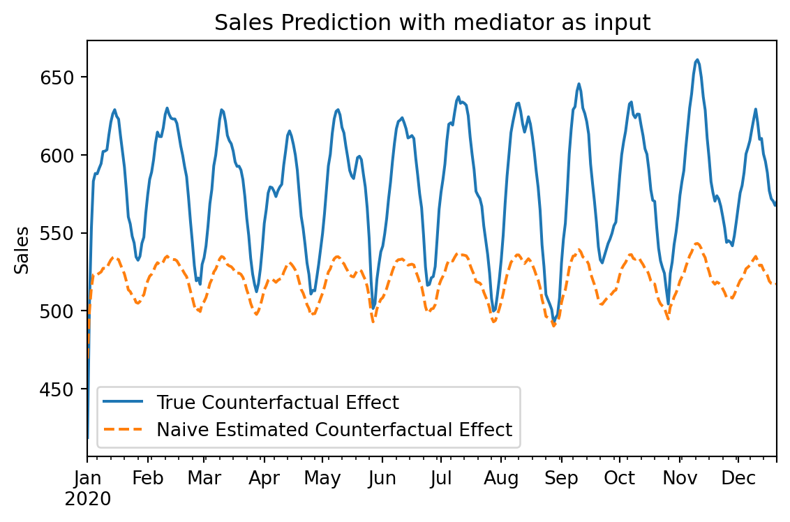

As we can see, the naive model significantly underestimates the effect of investment. It attributes the sales to visits, ignoring that investment caused those visits.

Front-door adjustment model

To correctly estimate the effect of investment while utilizing the data from visits, we need to model the causal structure. This is often called a Front-door adjustment or simply structural modeling.

In Prophetverse, we can achieve this by defining a Latent Variable for visits.

Latent Visits: We define latent/visits as a function of investment (plus trend/seasonality). This represents the “expected visits” given the investment.
Coupling: We link this latent/visits to the observed visits data using CoupledExactLikelihood. This tells the model: “The latent/visits variable should be close to the observed visits data.”
Sales Model: We use latent/visits as an input to explain sales.

This way, investment is the source of the variation in latent/visits, which in turn explains sales. The model understands that investment causes sales through visits.

graph LR
    I[Investment] --> LV((Latent Visits))
    LV -.->|Coupled| V[Observed Visits]
    LV --> S[Sales]

Let’s implement this in Prophetverse.

model = Prophetverse(
    trend=FlatTrend(changepoint_prior_scale=1000),
    inference_engine=MAPInferenceEngine(progress_bar=True),
    exogenous_effects=[
        # Multiplicative seasonality
        seasonality,
        # Now, the investment creates a latent component of "visits"
        (
            "latent/visits",
            investment_saturation_adstock,
            exact("investment"),
        ),
        # We use identity to put the mediator as a latent component
        (
            "latent/visit_input",
            Identity(),
            exact("visits"),
        ),
        # Both latent components should be coupled
        (
            "latent/coupled_likelihood",
            CoupledExactLikelihood(
                source_effect_name="latent/visits",
                target_effect_name="latent/visit_input",
                prior_scale=0.1,
            ),
            None,
        ),
        # We then convert the latent component to sales
        (
            "visit_sales",
            MultiplyEffects(
                effects=[
                    ("awareness", Forward("latent/visits")),
                    (
                        "conversion",
                        Constant(prior=dist.Beta(2, 2)),
                    ),
                ]
            ),
            None,
        ),
    ],
    scale=1,
)


model.fit(y=y, X=X)

  0%|          | 0/1 [00:00<?, ?it/s]100%|██████████| 1/1 [00:06<00:00,  6.74s/it, init loss: 6336.8862, avg. loss [1-1]: 6336.8862]100%|██████████| 1/1 [00:06<00:00,  6.74s/it, init loss: 6336.8862, avg. loss [1-1]: 6336.8862]

delta_frontdoor = get_treatment_effect(model, X)

fig, ax = plt.subplots(figsize=(6, 4))
delta_true.plot(ax=ax, label="True Counterfactual Effect", color="C0")
delta_naive["sales"].plot(ax=ax, label="Naive Estimated Counterfactual Effect", color="C1", linestyle="--")
delta_frontdoor["sales"].plot(ax=ax, label="Front-door Estimated Counterfactual Effect", color="C2", linestyle="--")
ax.set_title("Sales Prediction with Front-door Adjustment")
ax.set_ylabel("Sales")
ax.legend()
plt.tight_layout()
plt.show()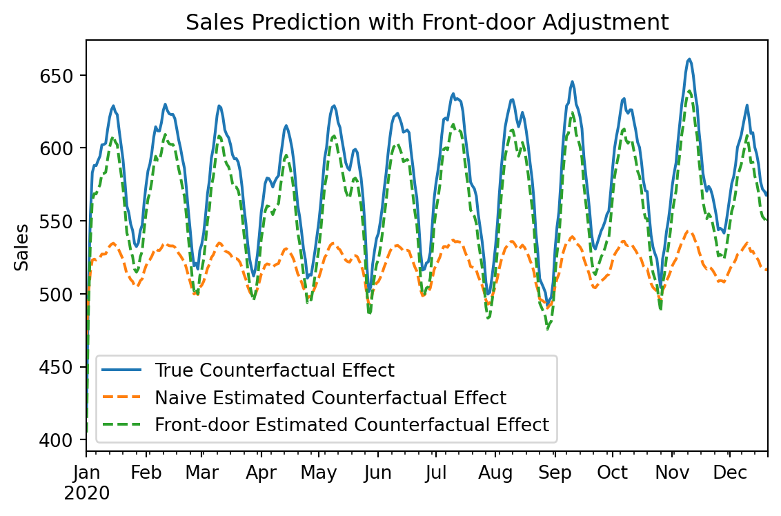

The plot above shows that the Front-door adjustment model (Green) recovers the True Counterfactual Effect (Blue) much better than the Naive model (Orange).

By explicitly modeling the mechanism Investment -> Visits -> Sales, we can:

Use the visits data to constrain the model and reduce uncertainty.
Correctly attribute the sales lift to the original investment.
Estimate the conversion rate from visits to sales separately from the effect of investment on visits.

This approach is powerful for MMM when you have rich funnel data and want to understand the full impact of your marketing activities.