import matplotlib.pyplot as plt
import numpy as np
import pandas as pd
from prophetverse.datasets.loaders import load_tourismHierarchical Bayesian Model
A tutorial demonstrating how to leverage hierarchical bayesian models to forecast panel timeseries
In this example, we will show how to forecast panel timeseries with the Prophetverse model.
The univariate Prophetverse model can seamlessly handle hierarchical timeseries due to the package’s compatibility with sktime.
Import dataset
Here we use the tourism dataset with purpose-level aggregation.
y = load_tourism(groupby="Purpose")
display(y)| Trips | ||
|---|---|---|
| Purpose | Quarter | |
| Business | 1998Q1 | 7391.962068 |
| 1998Q2 | 7701.153191 | |
| 1998Q3 | 8911.852065 | |
| 1998Q4 | 7777.766525 | |
| 1999Q1 | 6917.257864 | |
| ... | ... | ... |
| __total | 2015Q4 | 51518.858354 |
| 2016Q1 | 54984.720748 | |
| 2016Q2 | 49583.595515 | |
| 2016Q3 | 49392.159616 | |
| 2016Q4 | 54034.155613 |
380 rows × 1 columns
We define the helper function below to plot the predictions and the observations.
LEVELS = y.index.get_level_values(0).unique()


def plot_preds(y=None, preds={}, axs=None):

    if axs is None:
        fig, axs = plt.subplots(
            figsize=(12, 8), nrows=int(np.ceil(len(LEVELS) / 2)), ncols=2
        )
    ax_generator = iter(axs.flatten())
    for level in LEVELS:
        ax = next(ax_generator)
        if y is not None:
            y.loc[level].iloc[:, 0].rename("Observation").plot(
                ax=ax, label="truth", color="black"
            )
        for name, _preds in preds.items():
            _preds.loc[level].iloc[:, 0].rename(name).plot(ax=ax, legend=True)
        ax.set_title(level)

    # Tight layout
    plt.tight_layout()
    return ax
Automatic upcasting
Because of sktime’s amazing interface, we can use the univariate Prophet seamlessly with hierarchical data.
import jax.numpy as jnp

from prophetverse.effects import LinearFourierSeasonality
from prophetverse.effects.trend import PiecewiseLinearTrend, PiecewiseLogisticTrend
from prophetverse.engine import MAPInferenceEngine, MCMCInferenceEngine
from prophetverse.sktime.univariate import Prophetverse
from prophetverse.utils import no_input_columns
from prophetverse.engine.optimizer import LBFGSSolver

model = Prophetverse(
    trend=PiecewiseLogisticTrend(
        changepoint_prior_scale=0.1,
        changepoint_interval=8,
        changepoint_range=-8,
    ),
    exogenous_effects=[
        (
            "seasonality",
            LinearFourierSeasonality(
                sp_list=["YE"],
                fourier_terms_list=[1],
                freq="Q",
                prior_scale=0.1,
                effect_mode="multiplicative",
            ),
            no_input_columns,
        )
    ],
    inference_engine=MCMCInferenceEngine(
        num_warmup=500,
        num_samples=1000,
    ),
)
model.fit(y=y)
Prophetverse(exogenous_effects=[('seasonality',
LinearFourierSeasonality(effect_mode='multiplicative',
fourier_terms_list=[1],
freq='Q',
prior_scale=0.1,
sp_list=['YE']),
'^$')],
inference_engine=MCMCInferenceEngine(num_warmup=500),
trend=PiecewiseLogisticTrend(changepoint_interval=8,
changepoint_prior_scale=0.1,
changepoint_range=-8))Please rerun this cell to show the HTML repr or trust the notebook.Prophetverse(exogenous_effects=[('seasonality',
LinearFourierSeasonality(effect_mode='multiplicative',
fourier_terms_list=[1],
freq='Q',
prior_scale=0.1,
sp_list=['YE']),
'^$')],
inference_engine=MCMCInferenceEngine(num_warmup=500),
trend=PiecewiseLogisticTrend(changepoint_interval=8,
changepoint_prior_scale=0.1,
changepoint_range=-8))PiecewiseLogisticTrend(changepoint_interval=8, changepoint_prior_scale=0.1,
changepoint_range=-8)LinearFourierSeasonality(effect_mode='multiplicative', fourier_terms_list=[1],
freq='Q', prior_scale=0.1, sp_list=['YE'])MCMCInferenceEngine(num_warmup=500)
We can see how, internally, sktime creates clones of the model for each timeseries instance:
model.forecasters_| forecasters | |
|---|---|
| Business | Prophetverse(exogenous_effects=[('seasonality'... |
| Holiday | Prophetverse(exogenous_effects=[('seasonality'... |
| Other | Prophetverse(exogenous_effects=[('seasonality'... |
| Visiting | Prophetverse(exogenous_effects=[('seasonality'... |
| __total | Prophetverse(exogenous_effects=[('seasonality'... |
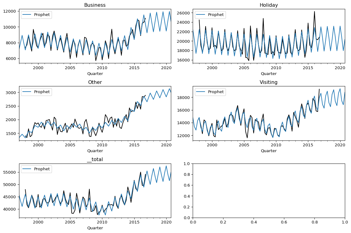
To call the same methods we used in the univariate case, we do not need to change a single line of code. The only difference is that the output will be a pd.DataFrame with more rows and index levels.
forecast_horizon = pd.period_range("1997Q1",
                                   "2020Q4",
                                   freq="Q")
preds = model.predict(fh=forecast_horizon)
display(preds.head())

# Plot
plot_preds(y, {"Prophet": preds})
plt.show()| Trips | ||
|---|---|---|
| Purpose | Quarter | |
| Business | 1997Q1 | 7063.018066 |
| 1997Q2 | 7994.687988 | |
| 1997Q3 | 8913.973633 | |
| 1997Q4 | 7973.970703 | |
| 1998Q1 | 7063.018066 |
The same applies to the decomposition method:
decomposition = model.predict_components(fh=forecast_horizon)
decomposition.head()| mean | obs | seasonality | trend | ||
|---|---|---|---|---|---|
| Business | 1997Q1 | 7063.018066 | 7069.990234 | -925.290283 | 7988.311035 |
| 1997Q2 | 7994.687988 | 7956.177246 | 6.377407 | 7988.311035 | |
| 1997Q3 | 8913.973633 | 8932.326172 | 925.661804 | 7988.311035 | |
| 1997Q4 | 7973.970703 | 7947.738281 | -14.344183 | 7988.311035 | |
| 1998Q1 | 7063.018066 | 7048.376465 | -925.290283 | 7988.311035 |
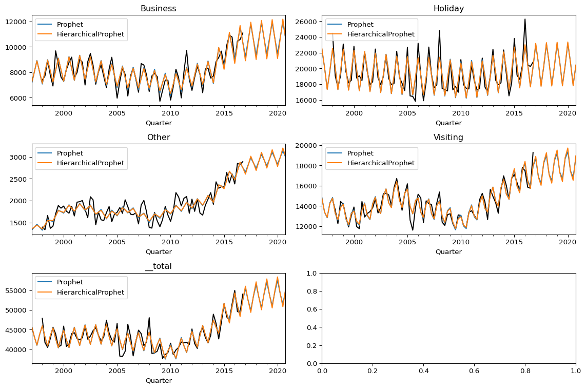
Hierarchical Bayesian model
Sometimes, we want to capture patterns shared between the different series, such as seasonality or trend. In this case, we can use a Bayesian Hierarchical Model.
A Bayesian Hierarchical Model sets hyperpriors: global priors over the priors for each timeseries. These hyperpriors allow us to share information across the different series, which can lead to better forecasts, especially when some series have very few observations.
To do that, we just need to use PanelBHLinearEffect as the seasonality__linear_effect parameter in the model. This effect will automatically create a hierarchical model for the linear effects, allowing us to share information across the different series. Also, let us set the broadcast_mode to “off” to use a single model to all the series.
from prophetverse.effects.linear import PanelBHLinearEffect

from numpyro import distributions as dist

model_hier = model.clone()
model_hier.set_params(
    seasonality__linear_effect=PanelBHLinearEffect(
        scale_hyperprior=dist.HalfNormal(0.1)
    ),
    broadcast_mode="effect",
)
model_hier.fit(y=y)
Prophetverse(broadcast_mode='effect',
exogenous_effects=[('seasonality',
LinearFourierSeasonality(effect_mode='multiplicative',
fourier_terms_list=[1],
freq='Q',
linear_effect=PanelBHLinearEffect(scale_hyperprior=<numpyro.distributions.continuous.HalfNormal object at 0x7f8a43f1fc50 with batch shape () and event shape ()>),
prior_scale=0.1,
sp_list=['YE']),
'^$')],
inference_engine=MCMCInferenceEngine(num_warmup=500),
trend=PiecewiseLogisticTrend(changepoint_interval=8,
changepoint_prior_scale=0.1,
changepoint_range=-8))Please rerun this cell to show the HTML repr or trust the notebook.Prophetverse(broadcast_mode='effect',
exogenous_effects=[('seasonality',
LinearFourierSeasonality(effect_mode='multiplicative',
fourier_terms_list=[1],
freq='Q',
linear_effect=PanelBHLinearEffect(scale_hyperprior=<numpyro.distributions.continuous.HalfNormal object at 0x7f8a43f1fc50 with batch shape () and event shape ()>),
prior_scale=0.1,
sp_list=['YE']),
'^$')],
inference_engine=MCMCInferenceEngine(num_warmup=500),
trend=PiecewiseLogisticTrend(changepoint_interval=8,
changepoint_prior_scale=0.1,
changepoint_range=-8))PiecewiseLogisticTrend(changepoint_interval=8, changepoint_prior_scale=0.1,
changepoint_range=-8)LinearFourierSeasonality(effect_mode='multiplicative', fourier_terms_list=[1],
freq='Q',
linear_effect=PanelBHLinearEffect(scale_hyperprior=<numpyro.distributions.continuous.HalfNormal object at 0x7f8a43f1fc50 with batch shape () and event shape ()>),
prior_scale=0.1, sp_list=['YE'])PanelBHLinearEffect(scale_hyperprior=<numpyro.distributions.continuous.HalfNormal object at 0x7f8a43f1fc50 with batch shape () and event shape ()>)
PanelBHLinearEffect(scale_hyperprior=<numpyro.distributions.continuous.HalfNormal object at 0x7f8a43f1fc50 with batch shape () and event shape ()>)
MCMCInferenceEngine(num_warmup=500)
preds_hier = model_hier.predict(fh=forecast_horizon)

plot_preds(
    y,
    preds={
        "Prophet": preds,
        "HierarchicalProphet": preds_hier,
    },
)