Composition of effects

This guide explains how to create effects that use the output of other effects.

In previous examples, we saw how to create a simple custom effect, which applies a simple transformation to the input data. However, the effect’s interface allows us to apply more complex transformations, such as using the output of previous components as input for the current component, or creating a composite effect that wraps an effect and applies some sort of transformation. This example will cover these topics.

Creating a custom effect

The idea here is to create an effect that uses another predicted component to scale the impact of an exogenous variable.

One classic use-case for this would be using seasonality to scale the effect of investment, that might be proportional to it. Marketing investments are a good example of this. We will implement such a composite effect in this section.

Example dataset

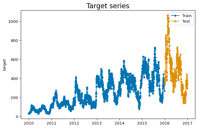
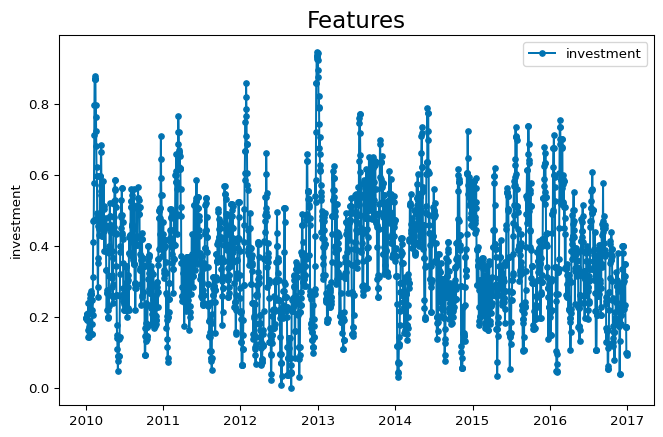
The dataset we use is synthetic, and the relation between the exogenous variable and the target is known. However, let’s pretend we don’t know this relation, and analize the data to find some insights that motivate the creation of a custom effect. The dataset has a target variable, which is a time series, and an exogenous variable, which is the investment made for each date.

import numpyro
import numpyro.distributions as dist
from matplotlib import pyplot as plt
from sktime.split import temporal_train_test_split
from sktime.utils.plotting import plot_series

from prophetverse.datasets.synthetic import load_composite_effect_example

numpyro.enable_x64()

y, X = load_composite_effect_example()

y_train, y_test, X_train, X_test = temporal_train_test_split(y, X, test_size=365)

display(y_train.head())
display(X_train.head())

/opt/hostedtoolcache/Python/3.11.12/x64/lib/python3.11/site-packages/tqdm/auto.py:21: TqdmWarning: IProgress not found. Please update jupyter and ipywidgets. See https://ipywidgets.readthedocs.io/en/stable/user_install.html
  from .autonotebook import tqdm as notebook_tqdm

	target
time
2010-01-01	29.375431
2010-01-02	30.268786
2010-01-03	29.128912
2010-01-04	31.014165
2010-01-05	31.890928

	investment
time
2010-01-01	0.198274
2010-01-02	0.198274
2010-01-03	0.198274
2010-01-04	0.198274
2010-01-05	0.207695

fig, ax = plt.subplots(figsize=(8,5))
plot_series(y_train, y_test, labels=["Train", "Test"], title="Target series", ax=ax)
fig.show()

fig, ax = plt.subplots(figsize=(8, 5))
plot_series(X["investment"], labels=["investment"], title="Features", ax=ax)
fig.show()

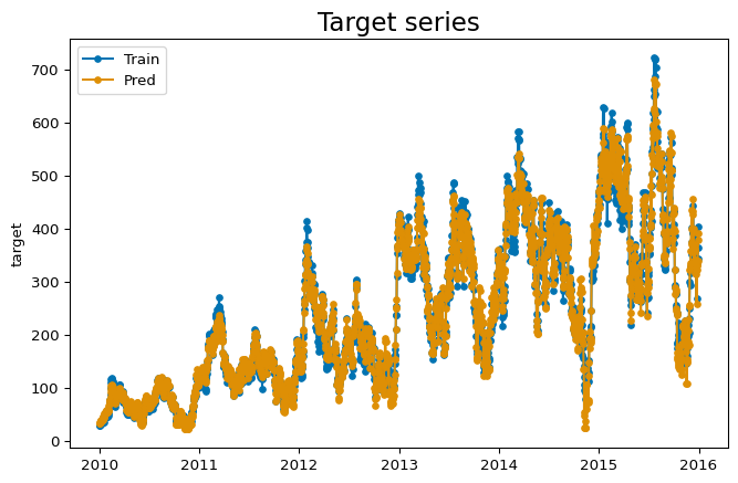
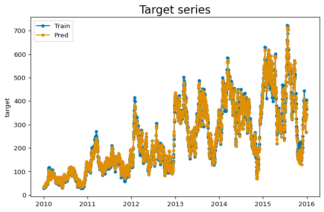
The timeseries has a yearly seasonality, and it seems that some oscillations are proportional to the investment. Below, we model the timeseries with a simple linear effect between the investment and the target, and a yearly seasonality based on fourier terms. Then, we will analize the residuals to see if there is any pattern that we can capture with a custom effect.

from prophetverse.effects import LinearEffect
from prophetverse.effects.fourier import LinearFourierSeasonality
from prophetverse.effects.trend import PiecewiseLinearTrend
from prophetverse.engine import MAPInferenceEngine
from prophetverse.engine.optimizer import LBFGSSolver
from prophetverse.sktime import Prophetverse
from prophetverse.utils.regex import exact, no_input_columns

model = Prophetverse(
    trend=PiecewiseLinearTrend(
        changepoint_interval=500,
        changepoint_prior_scale=0.00001,
        changepoint_range=-500,
    ),
    exogenous_effects=[
        (
            "seasonality",
            LinearFourierSeasonality(
                freq="D",
                sp_list=[365.25],
                fourier_terms_list=[5],
                prior_scale=1,
                effect_mode="multiplicative",
            ),
            no_input_columns,
        ),
        (
            "investment",
            LinearEffect("multiplicative", prior=dist.Normal(0, 1)),
            exact("investment"),
        ),
    ],
    inference_engine=MAPInferenceEngine(
        optimizer=LBFGSSolver(memory_size=100, max_linesearch_steps=100),
        progress_bar=True,
    ),
)

model.fit(y=y_train, X=X_train)
model

/home/runner/work/prophetverse/prophetverse/src/prophetverse/sktime/univariate.py:214: UserWarning: No columns match the regex ^$
  self._fit_effects(X, y)
  0%|          | 0/1 [00:00<?, ?it/s]100%|██████████| 1/1 [00:06<00:00,  6.08s/it, init loss: -5352.1071, avg. loss [1-1]: -5352.1071]100%|██████████| 1/1 [00:06<00:00,  6.08s/it, init loss: -5352.1071, avg. loss [1-1]: -5352.1071]

Prophetverse(exogenous_effects=[('seasonality',
                                 LinearFourierSeasonality(effect_mode='multiplicative',
                                                          fourier_terms_list=[5],
                                                          freq='D',
                                                          prior_scale=1,
                                                          sp_list=[365.25]),
                                 '^$'),
                                ('investment',
                                 LinearEffect(prior=<numpyro.distributions.continuous.Normal object at 0x7fc1b7af7ad0 with batch shape () and event shape ()>),
                                 '^investment$')],
             inference_engine=MAPInferenceEngine(optimizer=LBFGSSolver(max_linesearch_steps=100,
                                                                       memory_size=100),
                                                 progress_bar=True),
             trend=PiecewiseLinearTrend(changepoint_interval=500,
                                        changepoint_prior_scale=1e-05,
                                        changepoint_range=-500))

Please rerun this cell to show the HTML repr or trust the notebook.

We plot the predictions on training set to see if the model performs well.

y_pred = model.predict(X=X_train, fh=y_train.index)

fig, ax = plt.subplots(figsize=(8, 5))
plot_series(y_train, y_pred, labels=["Train", "Pred"], title="Target series", ax=ax)
fig.show()

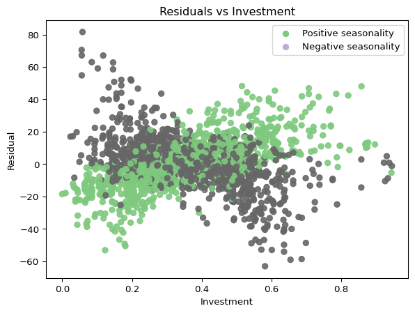
We can see that some peaks are not captured by the model. Our hypothesis to explain this phenomenon is that the investment has more impact on the target when it is done during the positive seasonality periods. To test this, we plot the residuals of the model against the investment, and color the points based on the seasonality component. We can see that slopes are different for positive and negative seasonality, which indicates that our hypothesis is possibly correct.

components = model.predict_components(X=X_train, fh=y_train.index)

residual = y_train["target"] - components["mean"]

fig, ax = plt.subplots()
ax.scatter(
    X_train["investment"],
    residual,
    c=components["seasonality"] < 0,
    cmap="Accent",
    alpha=0.9,
)
# Create legend manually
colors = plt.cm.get_cmap("Accent").colors
ax.scatter([], [], color=colors[0], label="Positive seasonality")
ax.scatter([], [], color=colors[1], label="Negative seasonality")
ax.legend()
ax.set(xlabel="Investment", ylabel="Residual", title="Residuals vs Investment")
fig.show()

/tmp/ipykernel_3880/182972736.py:14: MatplotlibDeprecationWarning: The get_cmap function was deprecated in Matplotlib 3.7 and will be removed in 3.11. Use ``matplotlib.colormaps[name]`` or ``matplotlib.colormaps.get_cmap()`` or ``pyplot.get_cmap()`` instead.
  colors = plt.cm.get_cmap("Accent").colors

Creating the composite effect

To model this behaviour with Prophetverse, we will create a custom effect, that scales a new effect by the output of a previous component. The _fit and _transform methods call the inner effect’s methods, and the predict method multiplies the inner effect’s predictions by the seasonality, which is passed as base_effect_name.

from typing import Any, Dict, List

import jax.numpy as jnp
import pandas as pd

from prophetverse.effects.base import BaseEffect


class WrapEffectAndScaleByAnother(BaseEffect):
    """Wrap an effect and scale it by another effect.

    Parameters
    ----------
    effect : BaseEffect
        The effect to wrap.

    """

    _tags = {"requires_X": False, "capability:panel": False}

    def __init__(
        self,
        effect: BaseEffect,
        base_effect_name: str,
    ):

        self.effect = effect
        self.base_effect_name = base_effect_name

        super().__init__()

        self.clone_tags(effect)

    def _fit(self, y: pd.DataFrame, X: pd.DataFrame, scale: float = 1):
        """Initialize the effect."""
        self.effect.fit(X=X, y=y, scale=scale)

    def _transform(self, X: pd.DataFrame, fh: pd.Index) -> Dict[str, Any]:
        """Prepare input data to be passed to numpyro model."""
        return self.effect.transform(X=X, fh=fh)

    def _predict(
        self, data: Dict, predicted_effects: Dict[str, jnp.ndarray], *args, **kwargs
    ) -> jnp.ndarray:
        """Apply and return the effect values."""
        out = self.effect.predict(data=data, predicted_effects=predicted_effects)

        base_effect = predicted_effects[self.base_effect_name]
        return base_effect * out

Instantiating the model with the composite effect

To create the model, we use the model instance we have, and the rshift operator to append the composite effect to the model.

import numpyro.distributions as dist
from prophetverse.engine.optimizer import AdamOptimizer

composite_effect_tuple = (
    "investment_seasonality",  # The effect ID, can be what you want
    WrapEffectAndScaleByAnother(
        effect=LinearEffect("multiplicative", prior=dist.HalfNormal(1)),
        base_effect_name="seasonality",
    ),
    exact("investment"),
)


# We use the rshift operator to append an effect to the model
model_composite = model >> composite_effect_tuple

model_composite.fit(y=y_train, X=X_train)
y_pred_composite = model_composite.predict(X=X_train, fh=y_train.index)

/home/runner/work/prophetverse/prophetverse/src/prophetverse/sktime/univariate.py:214: UserWarning: No columns match the regex ^$
  self._fit_effects(X, y)
/home/runner/work/prophetverse/prophetverse/src/prophetverse/sktime/univariate.py:214: UserWarning: Columns {'investment'} are already set
  self._fit_effects(X, y)
  0%|          | 0/1 [00:00<?, ?it/s]100%|██████████| 1/1 [00:07<00:00,  7.44s/it, init loss: -6054.6937, avg. loss [1-1]: -6054.6937]100%|██████████| 1/1 [00:07<00:00,  7.45s/it, init loss: -6054.6937, avg. loss [1-1]: -6054.6937]

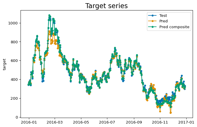
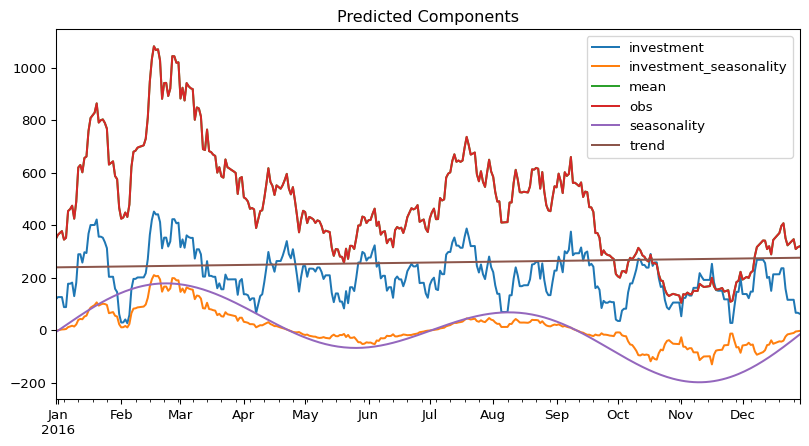
We can see below how these oscilations are captured by the model correctly when adding this joint effect.

fig, ax = plt.subplots(figsize=(8, 5))
plot_series(y_train, y_pred_composite, labels=["Train", "Pred"], title="Target series",ax=ax)
fig.show()

Evaluating the model on test set

We compare to the previous model to see if the new effect improved the predictions on test set:

y_pred_composite = model_composite.predict(X=X_test, fh=y_test.index)
y_pred = model.predict(X=X_test, fh=y_test.index)


fig, ax = plt.subplots(figsize=(8, 5))
plot_series(
    y_test,
    y_pred,
    y_pred_composite,
    labels=["Test", "Pred", "Pred composite"],
    title="Target series",
    ax=ax,
)

plt.show()

Extracting the components

The components can be extracted as usual, with the predict_components method.

components = model_composite.predict_components(fh=y_test.index, X=X_test)

fig, ax = plt.subplots(figsize=(10, 5))
components.plot.line(ax=ax)
ax.set_title("Predicted Components")
fig.show()