Saturation and Adstock

Learn how to use saturation and adstock transformations in Prophetverse to model diminishing returns and delayed effects of marketing activities.

There are many available effects available by default on Prophetverse. To get a glimpse of them, you can query all_objects from skbase.lookup:

from skbase.lookup import all_objects
from prophetverse.effects import BaseEffect

all_objects(object_types=[BaseEffect], package_name="prophetverse", as_dataframe=True)

/opt/hostedtoolcache/Python/3.11.13/x64/lib/python3.11/site-packages/tqdm/auto.py:21: TqdmWarning: IProgress not found. Please update jupyter and ipywidgets. See https://ipywidgets.readthedocs.io/en/stable/user_install.html
  from .autonotebook import tqdm as notebook_tqdm

	name	object
0	BetaTargetLikelihood	<class 'prophetverse.effects.target.univariate...
1	ChainedEffects	<class 'prophetverse.effects.chain.ChainedEffe...
2	Constant	<class 'prophetverse.effects.constant.Constant'>
3	ExactLikelihood	<class 'prophetverse.effects.exact_likelihood....
4	FlatTrend	<class 'prophetverse.effects.trend.flat.FlatTr...
5	GammaTargetLikelihood	<class 'prophetverse.effects.target.univariate...
6	GeometricAdstockEffect	<class 'prophetverse.effects.adstock.Geometric...
7	HillEffect	<class 'prophetverse.effects.hill.HillEffect'>
8	HurdleTargetLikelihood	<class 'prophetverse.effects.target.hurdle.Hur...
9	IgnoreInput	<class 'prophetverse.effects.ignore_input.Igno...
10	LiftExperimentLikelihood	<class 'prophetverse.effects.lift_likelihood.L...
11	LinearEffect	<class 'prophetverse.effects.linear.LinearEffe...
12	LinearFourierSeasonality	<class 'prophetverse.effects.fourier.LinearFou...
13	LogEffect	<class 'prophetverse.effects.log.LogEffect'>
14	MichaelisMentenEffect	<class 'prophetverse.effects.michaelis_menten....
15	MultiplyEffects	<class 'prophetverse.effects.multiply.Multiply...
16	MultivariateNormal	<class 'prophetverse.effects.target.multivaria...
17	NegativeBinomialTargetLikelihood	<class 'prophetverse.effects.target.univariate...
18	NormalTargetLikelihood	<class 'prophetverse.effects.target.univariate...
19	PanelBHLinearEffect	<class 'prophetverse.effects.linear.PanelBHLin...
20	PiecewiseLinearTrend	<class 'prophetverse.effects.trend.piecewise.P...
21	PiecewiseLogisticTrend	<class 'prophetverse.effects.trend.piecewise.P...
22	TargetLikelihood	<class 'prophetverse.effects.target.univariate...
23	WeibullAdstockEffect	<class 'prophetverse.effects.adstock.WeibullAd...

Not bad, right? The best part is that you can combine them in a flexible way to create your own custom effects, and even create your own effects if you want to. Below, we showcase some interesting combinations you can use, and how to visualize their prior predictive distribution.

Loading the dataset

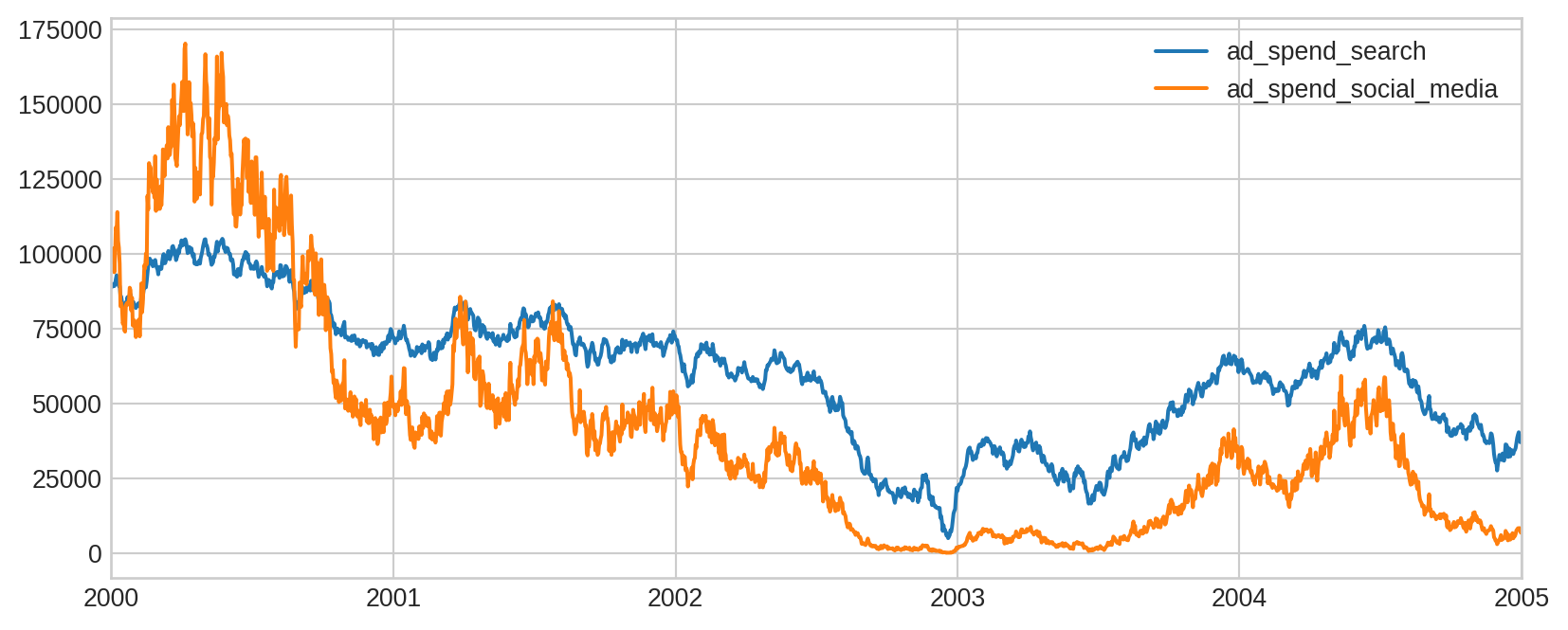
We load a synthetic dataset with daily frequency, to use in this example.

import matplotlib.pyplot as plt
from prophetverse.datasets._mmm.dataset1 import get_dataset

y, X = get_dataset(return_y_and_X_only=True)


y.head()

2000-01-01    10815512.0
2000-01-02    11120677.0
2000-01-03    11260387.0
2000-01-04    11322533.0
2000-01-05    11321180.0
Freq: D, dtype: float32

fig, ax = plt.subplots(figsize=(10, 4))
X.plot.line(ax=ax)
fig.show()

Saturations

The most common saturation functions are Hill, Michaelis-Menten, and Logarithmic. They are all available in Prophetverse:

from prophetverse.effects import MichaelisMentenEffect, HillEffect, LogEffect
import numpyro
from numpyro import distributions as dist

mm_saturation = MichaelisMentenEffect(
    effect_mode="additive",
    max_effect_prior=dist.HalfNormal(0.4),
    half_saturation_prior=dist.HalfNormal(40000),
)

log_saturation = LogEffect(
    effect_mode="additive",
    scale_prior=dist.HalfNormal(0.2),
    rate_prior=dist.HalfNormal(0.0001),
)

hill_saturation = HillEffect(
    effect_mode="additive",
    max_effect_prior=dist.HalfNormal(0.4),
    half_max_prior=dist.HalfNormal(40000),
    slope_prior=dist.InverseGamma(4, 2),
)

mm_saturation

MichaelisMentenEffect(effect_mode='additive',
                      half_saturation_prior=<numpyro.distributions.continuous.HalfNormal object at 0x7fdad43696d0 with batch shape () and event shape ()>,
                      max_effect_prior=<numpyro.distributions.continuous.HalfNormal object at 0x7fdad8a85c50 with batch shape () and event shape ()>)

Please rerun this cell to show the HTML repr or trust the notebook.

Tip

Since Prophetverse and all effects are estimators, you can set and inspect the hyperparameters through get_params and set_params methods, and of course plug them into an automated hyperparameter tuning workflow. Checkout our Hyperparameter Tuning tutorial for more details.

Visualizing prior predictive distributions

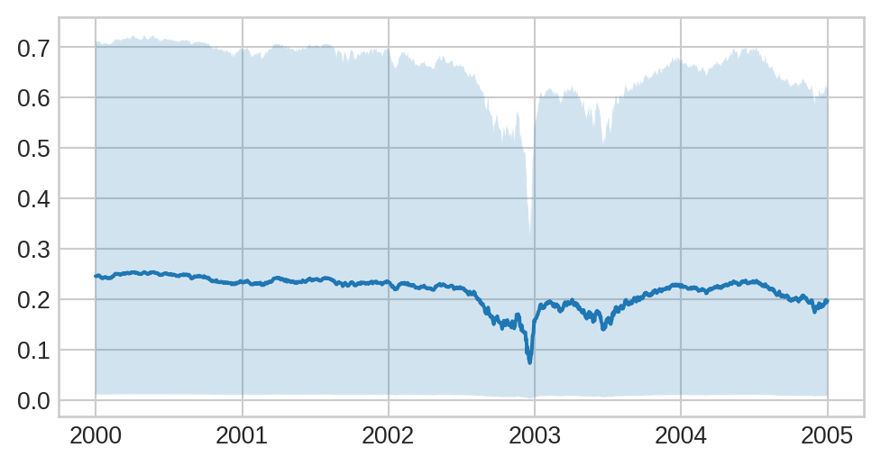
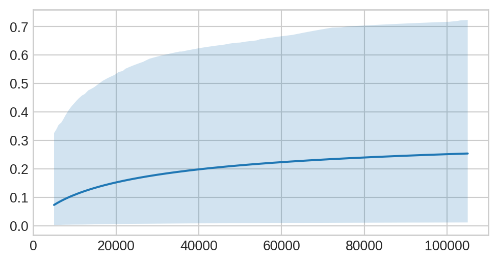
To get a better sense of how these effects behave, we can visualize their prior predictive distributions using the plot_prior_predictive utility from prophetverse.utils.plotting.

We first visualize how the output of the effect behaves with respect to the input:

from prophetverse.utils.plotting import plot_prior_predictive
import matplotlib.pyplot as plt


fig, ax = plot_prior_predictive(
    mm_saturation,
    X=X[["ad_spend_search"]],
    mode="ad_spend_search",
    matplotlib_kwargs=dict(figsize=(6, 3)),
)

fig.show()

And through time, when applied to a time series:

fig, ax = plot_prior_predictive(
    mm_saturation,
    X=X[["ad_spend_search"]],
    mode="time",
    matplotlib_kwargs=dict(figsize=(6, 3)),
)
fig.show()

Adstock

To model the delayed effect of advertising on sales, we can use adstock transformations.

Let’s visualize first how Weibull Adstock behaves when applied to the input:

from prophetverse import GeometricAdstockEffect, WeibullAdstockEffect

adstock = WeibullAdstockEffect(
    scale_prior=dist.HalfNormal(10),
    concentration_prior=dist.HalfNormal(2),
)

fig, ax = plot_prior_predictive(
    adstock,
    X=X[["ad_spend_search"]].iloc[100:180],
    mode="time",
    matplotlib_kwargs=dict(figsize=(6, 3)),
)
X[["ad_spend_search"]].iloc[100:180].plot(ax=ax, color="tab:orange")

for line, label in zip(ax.lines, ["After Adstock", "Input Data"]):
    line.set_label(label)
ax.legend()
fig.show()

And how Geometric Adstock behaves:

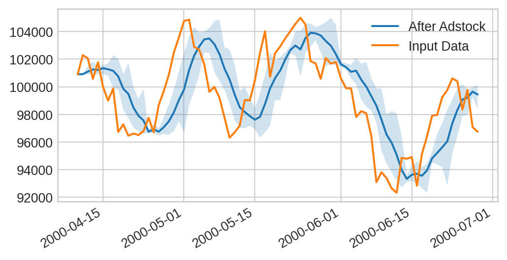
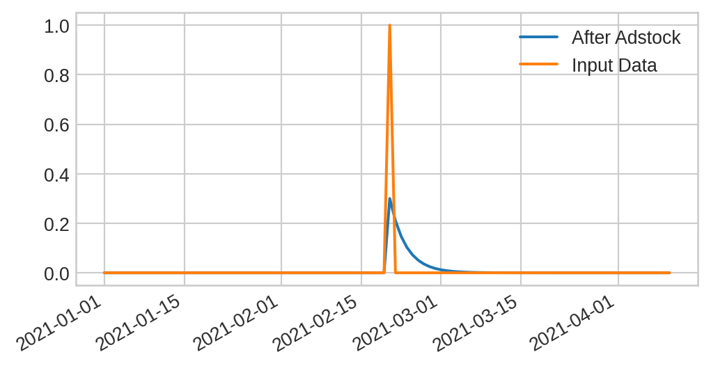
adstock = GeometricAdstockEffect(
    decay_prior=dist.Beta(10, 10),
    # Set normalize=True if you want an impulse of size 1 to have total
    # cumulative mass 1 over infinite horizon (weights sum to 1)
    normalize=True,
)

fig, ax = plot_prior_predictive(
    adstock,
    X=X[["ad_spend_search"]],
    mode="time",
    matplotlib_kwargs=dict(figsize=(6, 3)),
)
X[["ad_spend_search"]].plot(ax=ax, color="tab:orange")


ax.set(xlim=("2000-04-15", "2000-07-15"), ylim=(80_000, 110_000))

for line, label in zip(ax.lines, ["After Adstock", "Input Data"]):
    line.set_label(label)
ax.legend()
fig.show()

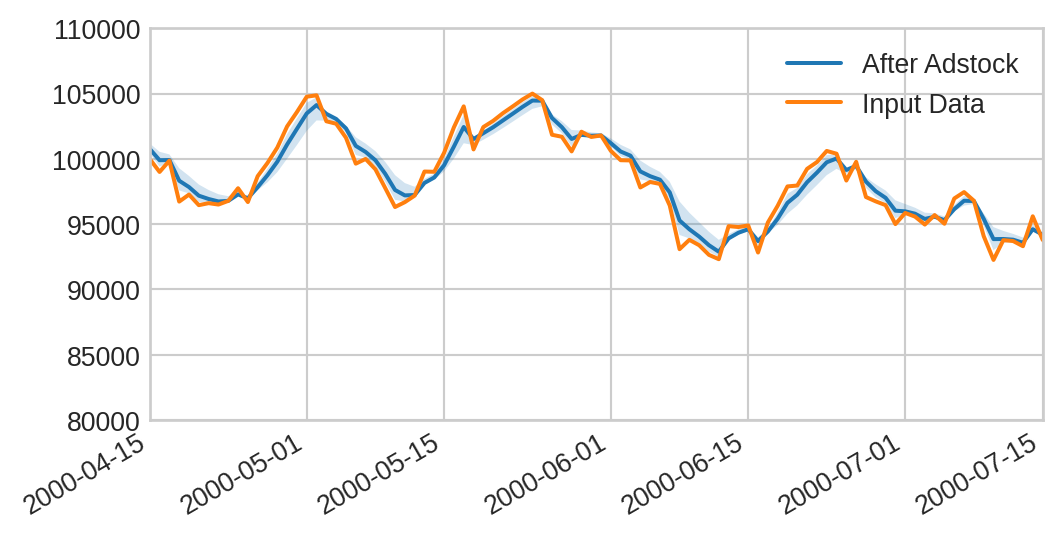
Combining Saturation and Adstock

And you can of course compose them! Use ChainedEffects to combine multiple effects in a sequence. Below, we combine Michaelis-Menten saturation with Weibull Adstock. You

from prophetverse import ChainedEffects

saturation_with_adstock = ChainedEffects(
    steps=[
        (
            "adstock_on_investment",
            WeibullAdstockEffect(
                scale_prior=dist.HalfNormal(2),
                concentration_prior=dist.HalfNormal(2),
            ),
        ),
        ("saturation", mm_saturation),
        (
            "adstock_on_output",
            WeibullAdstockEffect(
                scale_prior=dist.HalfNormal(2),
                concentration_prior=dist.HalfNormal(2),
            ),
        ),
    ]
)

saturation_with_adstock

ChainedEffects(steps=[('adstock_on_investment',
                       WeibullAdstockEffect(concentration_prior=<numpyro.distributions.continuous.HalfNormal object at 0x7fdad40d2490 with batch shape () and event shape ()>,
                                            scale_prior=<numpyro.distributions.continuous.HalfNormal object at 0x7fdad8a6ef10 with batch shape () and event shape ()>)),
                      ('saturation',
                       MichaelisMentenEffect(effect_mode='a...
                                             max_effect_prior=<numpyro.distributions.continuous.HalfNormal object at 0x7fdad8a85c50 with batch shape () and event shape ()>)),
                      ('adstock_on_output',
                       WeibullAdstockEffect(concentration_prior=<numpyro.distributions.continuous.HalfNormal object at 0x7fda96e8d990 with batch shape () and event shape ()>,
                                            scale_prior=<numpyro.distributions.continuous.HalfNormal object at 0x7fdad88b2f90 with batch shape () and event shape ()>))])

Please rerun this cell to show the HTML repr or trust the notebook.

fig, ax = plot_prior_predictive(
    mm_saturation,
    X=X[["ad_spend_search"]],
    mode="ad_spend_search",
    matplotlib_kwargs=dict(figsize=(6, 3)),
)
fig.show()

Extra: Visualizing the impulse response of adstock

The impulse response is one of the clearest ways to understand what adstock is doing.
By feeding in a single one-day spike of spend (an impulse), we can isolate the effect of the adstock transformation without confounding from the full time series.

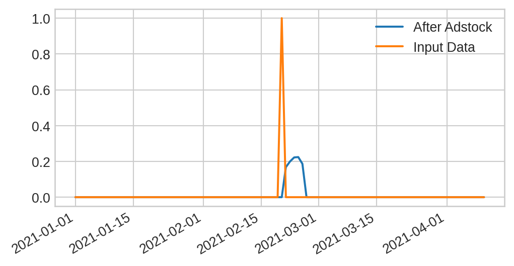
• Isolates carryover → shows exactly how much of today’s spend impacts tomorrow and the following days.
  
• Builds intuition → a short tail means fast decay; a long tail means the campaign keeps influencing for weeks.
  
• Compares models → geometric adstock has an exponential-like drop, while Weibull can flexibly capture rises before decay.
  
• Business meaning → directly answers “If I invest 1 unit today, what incremental impact should I expect tomorrow, next week, and beyond?”

In short, the impulse response is the “fingerprint” of an adstock model — it makes lag and memory structures visible and interpretable.

import pandas as pd


def plot_impulse_response(adstock):
    X_impulse = pd.DataFrame(
        index=pd.period_range(start="2021-01-01", periods=100, freq="D"),
        data=[0] * 50 + [1] + [0] * 49,
    ).astype(float)

    fig, ax = plot_prior_predictive(
        adstock,
        X=X_impulse,
        mode="time",
        matplotlib_kwargs=dict(figsize=(6, 3)),
    )
    X_impulse.plot(ax=ax, color="tab:orange")
    for line, label in zip(ax.lines, ["After Adstock", "Input Data"]):
        line.set_label(label)
    ax.legend()
    fig.show()


adstock = GeometricAdstockEffect(
    decay_prior=dist.Delta(0.7),
    normalize=True,
)
plot_impulse_response(adstock)

And for Weibull Adstock:

adstock = WeibullAdstockEffect(
    scale_prior=dist.Delta(5),
    concentration_prior=dist.Delta(1.5),
)
plot_impulse_response(adstock)