import numpy as np
import pandas as pd
import matplotlib.pyplot as plt
import numpyro
import numpyro.distributions as dist

plt.style.use("seaborn-v0_8-whitegrid")
numpyro.enable_x64()Forecasting, Calibration, and Unified Marketing Measurement
A tutorial on building a Marketing Mix Model (MMM) with Prophetverse, including forecasting, calibration, and unified marketing measurement.
In this tutorial, we walk through the lifecycle of a modern Marketing Mix Model (MMM), from time-series forecasting to incorporating causal evidence like lift tests and attribution.
You will learn:
- How to forecast revenue using media spend with Adstock and Saturation effects.
- How to diagnose model behavior and evaluate with backtesting.
- Why correlated spend channels confuse effect estimation—and how to fix it.
- How to calibrate your model using lift tests and attribution models for better ROI measurement.
👉 Why this matters: MMMs are foundational for budget allocation. But good predictions are not enough — we need credible effect estimates to make real-world decisions.
Let’s get started!
Setting up some libraries, float64 precision, and plot style:
from prophetverse.datasets._mmm.dataset1 import get_dataset

y, X, lift_tests, true_components, _ = get_dataset()
lift_test_search, lift_test_social = lift_tests

print(f"y shape: {y.shape}, X shape: {X.shape}")
X.head()
y shape: (1828,), X shape: (1828, 2)| ad_spend_search | ad_spend_social_media | |
|---|---|---|
| 2000-01-01 | 89076.191178 | 98587.488958 |
| 2000-01-02 | 88891.993106 | 99066.321168 |
| 2000-01-03 | 89784.955064 | 97334.106903 |
| 2000-01-04 | 89931.220681 | 101747.300585 |
| 2000-01-05 | 89184.319596 | 93825.221809 |
Part 1: Forecasting with Adstock & Saturation Effects
Here we’ll build a time-series forecasting model that includes:
- Trend and seasonality
- Lagged media effects (Adstock)
- Diminishing returns (Saturation / Hill curves)
🔎 Why this matters:
Raw spend is not immediately effective, and it doesn’t convert linearly.
Capturing these dynamics is essential to make ROI estimates realistic.
from prophetverse.effects import (
    PiecewiseLinearTrend,
    LinearFourierSeasonality,
    ChainedEffects,
    GeometricAdstockEffect,
    HillEffect,
)
from prophetverse.sktime import Prophetverse
from prophetverse.engine import MAPInferenceEngine
from prophetverse.engine.optimizer import LBFGSSolver

yearly = (
    "yearly_seasonality",
    LinearFourierSeasonality(freq="D", sp_list=[365.25], fourier_terms_list=[5], prior_scale=0.1, effect_mode="multiplicative"),
    None,
)

weekly = (
    "weekly_seasonality",
    LinearFourierSeasonality(freq="D", sp_list=[7], fourier_terms_list=[3], prior_scale=0.05, effect_mode="multiplicative"),
    None,
)

hill = HillEffect(
    half_max_prior=dist.HalfNormal(1),
    slope_prior=dist.InverseGamma(2, 1),
    max_effect_prior=dist.HalfNormal(1),
    effect_mode="additive",
    input_scale=1e6,
)

chained_search = (
    "ad_spend_search",
    ChainedEffects([("adstock", GeometricAdstockEffect()), ("saturation", hill)]),
    "ad_spend_search",
)
chained_social = (
    "ad_spend_social_media",
    ChainedEffects([("adstock", GeometricAdstockEffect()), ("saturation", hill)]),
    "ad_spend_social_media",
)
baseline_model = Prophetverse(
trend=PiecewiseLinearTrend(changepoint_interval=100),
exogenous_effects=[yearly, weekly, chained_search, chained_social],
inference_engine=MAPInferenceEngine(
num_steps=5000,
optimizer=LBFGSSolver(memory_size=300, max_linesearch_steps=300),
),
)
baseline_model.fit(y=y, X=X)Prophetverse(exogenous_effects=[('yearly_seasonality',
LinearFourierSeasonality(effect_mode='multiplicative',
fourier_terms_list=[5],
freq='D',
prior_scale=0.1,
sp_list=[365.25]),
None),
('weekly_seasonality',
LinearFourierSeasonality(effect_mode='multiplicative',
fourier_terms_list=[3],
freq='D',
prior_scale=0.05,
sp_list=[7]),
None),
('ad_spend_search',
Chained...
max_effect_prior=<numpyro.distributions.continuous.HalfNormal object at 0x7f0b90b2c390 with batch shape () and event shape ()>,
slope_prior=<numpyro.distributions.continuous.InverseGamma object at 0x7f0b4c6d3750 with batch shape () and event shape ()>))]),
'ad_spend_social_media')],
inference_engine=MAPInferenceEngine(num_steps=5000,
optimizer=LBFGSSolver(max_linesearch_steps=300,
memory_size=300)),
trend=PiecewiseLinearTrend(changepoint_interval=100))Please rerun this cell to show the HTML repr or trust the notebook.Prophetverse(exogenous_effects=[('yearly_seasonality',
LinearFourierSeasonality(effect_mode='multiplicative',
fourier_terms_list=[5],
freq='D',
prior_scale=0.1,
sp_list=[365.25]),
None),
('weekly_seasonality',
LinearFourierSeasonality(effect_mode='multiplicative',
fourier_terms_list=[3],
freq='D',
prior_scale=0.05,
sp_list=[7]),
None),
('ad_spend_search',
Chained...
max_effect_prior=<numpyro.distributions.continuous.HalfNormal object at 0x7f0b90b2c390 with batch shape () and event shape ()>,
slope_prior=<numpyro.distributions.continuous.InverseGamma object at 0x7f0b4c6d3750 with batch shape () and event shape ()>))]),
'ad_spend_social_media')],
inference_engine=MAPInferenceEngine(num_steps=5000,
optimizer=LBFGSSolver(max_linesearch_steps=300,
memory_size=300)),
trend=PiecewiseLinearTrend(changepoint_interval=100))PiecewiseLinearTrend(changepoint_interval=100)
LinearFourierSeasonality(effect_mode='multiplicative', fourier_terms_list=[5],
freq='D', prior_scale=0.1, sp_list=[365.25])LinearFourierSeasonality(effect_mode='multiplicative', fourier_terms_list=[3],
freq='D', prior_scale=0.05, sp_list=[7])ChainedEffects(steps=[('adstock', GeometricAdstockEffect()),
('saturation',
HillEffect(effect_mode='additive',
           half_max_prior=<numpyro.distributions.continuous.HalfNormal object at 0x7f0bbc7b1b10 with batch shape () and event shape ()>,
           input_scale=1000000.0,
           max_effect_prior=<numpyro.distributions.continuous.HalfNormal object at 0x7f0b90b2c390 with batch shape () and event shape ()>,
slope_prior=<numpyro.distributions.continuous.InverseGamma object at 0x7f0b4c6d3750 with batch shape () and event shape ()>))])GeometricAdstockEffect()
HillEffect(effect_mode='additive',
           half_max_prior=<numpyro.distributions.continuous.HalfNormal object at 0x7f0bbc7b1b10 with batch shape () and event shape ()>,
           input_scale=1000000.0,
           max_effect_prior=<numpyro.distributions.continuous.HalfNormal object at 0x7f0b90b2c390 with batch shape () and event shape ()>,
slope_prior=<numpyro.distributions.continuous.InverseGamma object at 0x7f0b4c6d3750 with batch shape () and event shape ()>)ChainedEffects(steps=[('adstock', GeometricAdstockEffect()),
('saturation',
HillEffect(effect_mode='additive',
half_max_prior=<numpyro.distributions.continuous.HalfNormal object at 0x7f0bbc7b1b10 with batch shape () and event shape ()>,
input_scale=1000000.0,
max_effect_prior=<numpyro.distributions.continuous.HalfNormal object at 0x7f0b90b2c390 with batch shape () and event shape ()>,
slope_prior=<numpyro.distributions.continuous.InverseGamma object at 0x7f0b4c6d3750 with batch shape () and event shape ()>))])GeometricAdstockEffect()
HillEffect(effect_mode='additive',
half_max_prior=<numpyro.distributions.continuous.HalfNormal object at 0x7f0bbc7b1b10 with batch shape () and event shape ()>,
input_scale=1000000.0,
max_effect_prior=<numpyro.distributions.continuous.HalfNormal object at 0x7f0b90b2c390 with batch shape () and event shape ()>,
slope_prior=<numpyro.distributions.continuous.InverseGamma object at 0x7f0b4c6d3750 with batch shape () and event shape ()>)MAPInferenceEngine(num_steps=5000,
optimizer=LBFGSSolver(max_linesearch_steps=300,
memory_size=300))y_pred = baseline_model.predict(X=X, fh=X.index)
plt.figure(figsize=(8, 4))
y.plot(label="Observed")
y_pred.plot(label="Predicted")
plt.title("In-Sample Forecast: Observed vs Predicted")
plt.legend()
plt.show()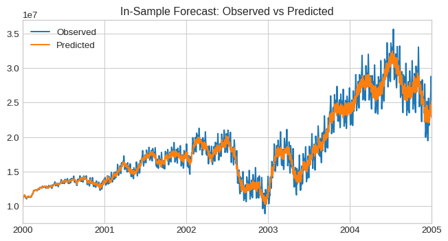
1.1 Component-Level Diagnostics
With predict_components, we can obtain the model’s components.
y_pred_components = baseline_model.predict_components(X=X, fh=X.index)
y_pred_components.head()| ad_spend_search | ad_spend_social_media | mean | obs | trend | weekly_seasonality | yearly_seasonality | |
|---|---|---|---|---|---|---|---|
| 2000-01-01 | 128.435246 | 9.934596e+06 | 1.013487e+07 | 1.011421e+07 | 215564.370674 | 9280.187211 | -24703.502867 |
| 2000-01-02 | 128.707328 | 1.075744e+07 | 1.095703e+07 | 1.091278e+07 | 224383.219339 | 363.501952 | -25286.638685 |
| 2000-01-03 | 128.805219 | 1.099429e+07 | 1.120473e+07 | 1.126298e+07 | 233202.068005 | 2901.752875 | -25784.368620 |
| 2000-01-04 | 128.847726 | 1.112811e+07 | 1.133260e+07 | 1.129217e+07 | 242020.916670 | -11466.408260 | -26191.575962 |
| 2000-01-05 | 128.865014 | 1.112434e+07 | 1.134729e+07 | 1.129867e+07 | 250839.765335 | -1515.730204 | -26503.361097 |
In a real use-casee, you would not have access to the ground truth of the components. We use them here to show how the model behaves, and how incorporing extra information can improve it.
fig, axs = plt.subplots(4, 1, figsize=(8, 12), sharex=True)
for i, name in enumerate(
    ["trend", "yearly_seasonality", "ad_spend_search", "ad_spend_social_media"]
):
    true_components[name].plot(ax=axs[i], label="True", color="black")
    y_pred_components[name].plot(ax=axs[i], label="Estimated")
    axs[i].set_title(name)
    axs[i].legend()
plt.tight_layout()
plt.show()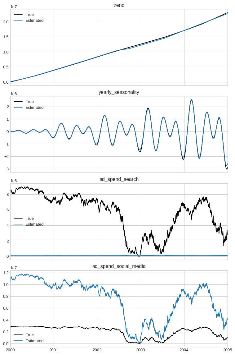
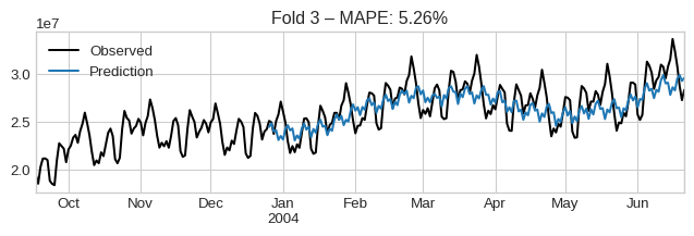
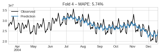
1.2 Backtesting with Cross-Validation
We use rolling-window CV to assess out-of-sample accuracy using MAPE.
🧠 Caution: Low error ≠ correct attribution. But high error often indicates a bad model.
from sktime.split import ExpandingWindowSplitter
from sktime.performance_metrics.forecasting import MeanAbsolutePercentageError
from sktime.forecasting.model_evaluation import evaluate

metric = MeanAbsolutePercentageError()
cv = ExpandingWindowSplitter(
    initial_window=365 * 3, step_length=180, fh=list(range(1, 180))
)
cv_results = evaluate(
    forecaster=baseline_model, y=y, X=X, cv=cv, scoring=metric, return_data=True
)
cv_results| test_MeanAbsolutePercentageError | fit_time | pred_time | len_train_window | cutoff | y_train | y_test | y_pred | |
|---|---|---|---|---|---|---|---|---|
| 0 | 0.066920 | 30.999431 | 0.874131 | 1095 | 2002-12-30 | 2000-01-01 1.081551e+07 2000-01-02 1.112... | 2002-12-31 1.306520e+07 2003-01-01 1.429... | 2002-12-31 1.116013e+07 2003-01-01 1.167... |
| 1 | 0.061507 | 88.793421 | 0.832869 | 1275 | 2003-06-28 | 2000-01-01 1.081551e+07 2000-01-02 1.112... | 2003-06-29 1.725815e+07 2003-06-30 1.696... | 2003-06-29 1.621793e+07 2003-06-30 1.648... |
| 2 | 0.052640 | 46.663078 | 0.847119 | 1455 | 2003-12-25 | 2000-01-01 1.081551e+07 2000-01-02 1.112... | 2003-12-26 2.511414e+07 2003-12-27 2.496... | 2003-12-26 2.447497e+07 2003-12-27 2.486... |
| 3 | 0.057910 | 26.413156 | 0.834119 | 1635 | 2004-06-22 | 2000-01-01 1.081551e+07 2000-01-02 1.112... | 2004-06-23 2.913561e+07 2004-06-24 2.878... | 2004-06-23 3.056416e+07 2004-06-24 3.018... |
The average error across folds is:
cv_results["test_MeanAbsolutePercentageError"].mean()np.float64(0.05974443208218553)We can visualize them by iterating the dataframe:
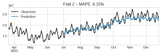
for idx, row in cv_results.iterrows():
    plt.figure(figsize=(8, 2))
    observed = pd.concat([row["y_train"].iloc[-100:], row["y_test"]])
    observed.plot(label="Observed", color="black")
    row["y_pred"].plot(label="Prediction")
    plt.title(f"Fold {idx + 1} – MAPE: {row['test_MeanAbsolutePercentageError']:.2%}")
    plt.legend()
    plt.show()
    if idx > 3:
        break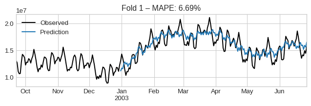
1.3 Saturation Curves
These curves show diminishing marginal effect as spend increases.
🔍 Insight: This shape helps guide budget allocation decisions (e.g. where additional spend will have little return).
Note how the model captures a saturation effect, but it is still far from the correct shape.
This is why, in many situations, you will need calibration to correct the model’s behavior. This is what we will do in the next section.
fig, axs = plt.subplots(figsize=(8, 6), nrows=1, ncols=2)

for ax, channel in zip(axs, ["ad_spend_search", "ad_spend_social_media"]):
    ax.scatter(
        X[channel],
        y_pred_components[channel],
        alpha=0.6,
        label=channel,
    )
    ax.scatter(
        X[channel],
        true_components[channel],
        color="black",
        label="True Effect",
    )
    ax.set(
        xlabel="Daily Spend",
        ylabel="Incremental Effect",
        title=f"{channel} - Saturation Curve",
    )
    ax.legend()

plt.tight_layout()
plt.show()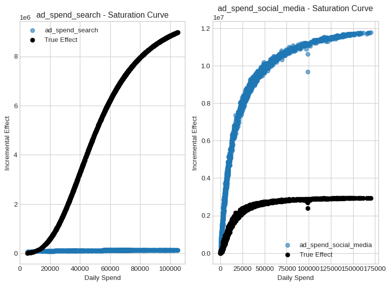
Part 2: Calibration with Causal Evidence
Time-series alone cannot disentangle correlated channels.
We integrate lift tests (local experiments) and attribution models (high-resolution signal) to correct this.
lift_test_search| lift | x_start | x_end | |
|---|---|---|---|
| 2000-09-04 | 0.986209 | 88991.849098 | 88616.674279 |
| 2003-07-17 | 1.602655 | 25147.476284 | 30137.721832 |
| 2004-04-11 | 0.762057 | 58323.761863 | 46723.500000 |
| 2003-01-06 | 0.758514 | 23857.995845 | 21913.505457 |
| 2003-03-07 | 1.332419 | 29036.114641 | 31676.191662 |
| 2001-01-17 | 1.142551 | 71184.337297 | 80915.848594 |
| 2003-04-12 | 1.654931 | 36588.754410 | 46777.071912 |
| 2002-02-16 | 0.825554 | 67892.914951 | 55030.729840 |
| 2001-10-05 | 0.929293 | 69504.770296 | 65128.356512 |
| 2000-10-02 | 0.994120 | 85176.526599 | 88936.541885 |
| 2003-06-05 | 0.760863 | 27988.449143 | 24654.281482 |
| 2000-07-07 | 0.897929 | 97458.154049 | 79856.919150 |
| 2003-09-28 | 1.570214 | 42328.076114 | 54497.175586 |
| 2002-08-24 | 0.863911 | 35824.789963 | 33256.068138 |
| 2000-11-28 | 1.242113 | 69593.024187 | 92943.044427 |
| 2001-12-28 | 0.881569 | 71500.973097 | 69504.085790 |
| 2001-09-02 | 1.197270 | 69966.800254 | 93695.953636 |
| 2002-12-16 | 1.660649 | 7810.413156 | 9322.237192 |
| 2004-08-30 | 1.286178 | 47599.593625 | 56735.271957 |
| 2001-02-18 | 1.254430 | 64837.275444 | 81784.074961 |
| 2000-05-15 | 1.044025 | 100464.794301 | 121779.610581 |
| 2004-08-13 | 0.967493 | 57864.200257 | 56080.324427 |
| 2001-02-02 | 1.212479 | 67857.642170 | 88071.282712 |
| 2001-05-21 | 1.178636 | 71337.927880 | 93445.016948 |
| 2003-05-06 | 0.644814 | 25609.287364 | 21843.082411 |
| 2000-07-31 | 1.012828 | 92617.293678 | 85766.681515 |
| 2002-07-03 | 1.267595 | 57443.596207 | 66595.562035 |
| 2004-09-27 | 1.369890 | 41546.443755 | 50176.823146 |
| 2000-10-25 | 0.985062 | 72757.343228 | 70195.986606 |
| 2002-11-02 | 0.834577 | 19043.272758 | 18373.397899 |
2.1 Visualizing Lift Tests
Each experiment records: pre-spend (x_start), post-spend (x_end), and measured lift. These give us causal “ground truth” deltas.
fig, ax = plt.subplots(figsize=(8, 6))

# Scatter plot for pre-spend and observed lift
ax.scatter(lift_test_search["x_start"], [1] * len(lift_test_search), label="Pre-Spend", alpha=0.6)
ax.scatter(lift_test_search["x_end"], lift_test_search["lift"], label="Observed Lift", alpha=0.6)

# Annotate with arrows to show lift effect
for _, row in lift_test_search.iterrows():
    ax.annotate(
        "",
        xy=(row["x_end"], row["lift"]),
        xytext=(row["x_start"], 1),
        arrowprops=dict(arrowstyle="->", alpha=0.5),
    )

# Add horizontal line and labels
ax.axhline(1, linestyle="--", color="gray", alpha=0.7)
ax.set(
    title="Search Ads Lift Tests",
    xlabel="Spend",
    ylabel="Revenue Ratio",
)

# Add legend and finalize layout
ax.legend()
plt.tight_layout()
plt.show()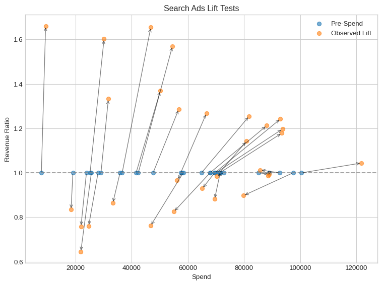
2.2 Improve Estimates via LiftExperimentLikelihood
This adds a new likelihood term that makes the model match lift observations.
🔁 Still Bayesian: It incorporates test variance and model uncertainty.
Since we use sktime interface, we have access to get_params() and set_params(**kwargs) methods. This allows us to easily swap effects and likelihoods. When we define our model, the effect’s name become a key in the model’s get_params() dictionary. We can use this to set the effect’s parameters directly.
from prophetverse.effects.lift_likelihood import LiftExperimentLikelihood

model_lift = baseline_model.clone()
model_lift.set_params(
    ad_spend_search=LiftExperimentLikelihood(
        effect=baseline_model.get_params()["ad_spend_search"],
        lift_test_results=lift_test_search,
        prior_scale=0.05,
    ),
    ad_spend_social_media=LiftExperimentLikelihood(
        effect=baseline_model.get_params()["ad_spend_social_media"],
        lift_test_results=lift_test_social,
        prior_scale=0.05,
    ),
)

model_lift.fit(y=y, X=X)
Prophetverse(exogenous_effects=[('yearly_seasonality',
LinearFourierSeasonality(effect_mode='multiplicative',
fourier_terms_list=[5],
freq='D',
prior_scale=0.1,
sp_list=[365.25]),
None),
('weekly_seasonality',
LinearFourierSeasonality(effect_mode='multiplicative',
fourier_terms_list=[3],
freq='D',
prior_scale=0.05,
sp_list=[7]),
None),
('ad_spend_search',
LiftExp...
2002-07-03 1.053316 25537.869750 38025.254409
2004-09-27 1.010456 8523.749415 11037.466255
2000-10-25 0.980559 50964.957119 65038.733878
2002-11-02 1.355164 1195.765141 1603.253926,
prior_scale=0.05),
'ad_spend_social_media')],
inference_engine=MAPInferenceEngine(num_steps=5000,
optimizer=LBFGSSolver(max_linesearch_steps=300,
memory_size=300)),
trend=PiecewiseLinearTrend(changepoint_interval=100))Please rerun this cell to show the HTML repr or trust the notebook.Prophetverse(exogenous_effects=[('yearly_seasonality',
LinearFourierSeasonality(effect_mode='multiplicative',
fourier_terms_list=[5],
freq='D',
prior_scale=0.1,
sp_list=[365.25]),
None),
('weekly_seasonality',
LinearFourierSeasonality(effect_mode='multiplicative',
fourier_terms_list=[3],
freq='D',
prior_scale=0.05,
sp_list=[7]),
None),
('ad_spend_search',
LiftExp...
2002-07-03 1.053316 25537.869750 38025.254409
2004-09-27 1.010456 8523.749415 11037.466255
2000-10-25 0.980559 50964.957119 65038.733878
2002-11-02 1.355164 1195.765141 1603.253926,
prior_scale=0.05),
'ad_spend_social_media')],
inference_engine=MAPInferenceEngine(num_steps=5000,
optimizer=LBFGSSolver(max_linesearch_steps=300,
memory_size=300)),
trend=PiecewiseLinearTrend(changepoint_interval=100))PiecewiseLinearTrend(changepoint_interval=100)
LinearFourierSeasonality(effect_mode='multiplicative', fourier_terms_list=[5],
freq='D', prior_scale=0.1, sp_list=[365.25])LinearFourierSeasonality(effect_mode='multiplicative', fourier_terms_list=[3],
freq='D', prior_scale=0.05, sp_list=[7])LiftExperimentLikelihood(effect=ChainedEffects(steps=[('adstock',
GeometricAdstockEffect()),
('saturation',
HillEffect(effect_mode='additive',
half_max_prior=<numpyro.distributions.continuous.HalfNormal object at 0x7f0bbc7b1b10 with batch shape () and event shape ()>,
input_scale=1000000.0,
max_effect_prior=<numpyro.distributions.continuous.HalfNormal object at 0x7f0b...
2001-02-02 1.212479 67857.642170 88071.282712
2001-05-21 1.178636 71337.927880 93445.016948
2003-05-06 0.644814 25609.287364 21843.082411
2000-07-31 1.012828 92617.293678 85766.681515
2002-07-03 1.267595 57443.596207 66595.562035
2004-09-27 1.369890 41546.443755 50176.823146
2000-10-25 0.985062 72757.343228 70195.986606
2002-11-02 0.834577 19043.272758 18373.397899,
prior_scale=0.05)ChainedEffects(steps=[('adstock', GeometricAdstockEffect()),
('saturation',
HillEffect(effect_mode='additive',
           half_max_prior=<numpyro.distributions.continuous.HalfNormal object at 0x7f0bbc7b1b10 with batch shape () and event shape ()>,
           input_scale=1000000.0,
           max_effect_prior=<numpyro.distributions.continuous.HalfNormal object at 0x7f0b90b2c390 with batch shape () and event shape ()>,
slope_prior=<numpyro.distributions.continuous.InverseGamma object at 0x7f0b4c6d3750 with batch shape () and event shape ()>))])GeometricAdstockEffect()
HillEffect(effect_mode='additive',
           half_max_prior=<numpyro.distributions.continuous.HalfNormal object at 0x7f0bbc7b1b10 with batch shape () and event shape ()>,
           input_scale=1000000.0,
           max_effect_prior=<numpyro.distributions.continuous.HalfNormal object at 0x7f0b90b2c390 with batch shape () and event shape ()>,
slope_prior=<numpyro.distributions.continuous.InverseGamma object at 0x7f0b4c6d3750 with batch shape () and event shape ()>)LiftExperimentLikelihood(effect=ChainedEffects(steps=[('adstock',
GeometricAdstockEffect()),
('saturation',
HillEffect(effect_mode='additive',
half_max_prior=<numpyro.distributions.continuous.HalfNormal object at 0x7f0bbc7b1b10 with batch shape () and event shape ()>,
input_scale=1000000.0,
max_effect_prior=<numpyro.distributions.continuous.HalfNormal object at 0x7f0b...
2001-02-02 1.085461 38129.336619 47626.107330
2001-05-21 0.961702 50010.574434 73721.957893
2003-05-06 1.099837 2893.044038 2702.425237
2000-07-31 1.028477 105196.357631 125200.174092
2002-07-03 1.053316 25537.869750 38025.254409
2004-09-27 1.010456 8523.749415 11037.466255
2000-10-25 0.980559 50964.957119 65038.733878
2002-11-02 1.355164 1195.765141 1603.253926,
prior_scale=0.05)ChainedEffects(steps=[('adstock', GeometricAdstockEffect()),
('saturation',
HillEffect(effect_mode='additive',
half_max_prior=<numpyro.distributions.continuous.HalfNormal object at 0x7f0bbc7b1b10 with batch shape () and event shape ()>,
input_scale=1000000.0,
max_effect_prior=<numpyro.distributions.continuous.HalfNormal object at 0x7f0b90b2c390 with batch shape () and event shape ()>,
slope_prior=<numpyro.distributions.continuous.InverseGamma object at 0x7f0b4c6d3750 with batch shape () and event shape ()>))])GeometricAdstockEffect()
HillEffect(effect_mode='additive',
half_max_prior=<numpyro.distributions.continuous.HalfNormal object at 0x7f0bbc7b1b10 with batch shape () and event shape ()>,
input_scale=1000000.0,
max_effect_prior=<numpyro.distributions.continuous.HalfNormal object at 0x7f0b90b2c390 with batch shape () and event shape ()>,
slope_prior=<numpyro.distributions.continuous.InverseGamma object at 0x7f0b4c6d3750 with batch shape () and event shape ()>)MAPInferenceEngine(num_steps=5000,
optimizer=LBFGSSolver(max_linesearch_steps=300,
memory_size=300))components_lift = model_lift.predict_components(X=X, fh=X.index)
components_lift.head()| ad_spend_search | ad_spend_social_media | mean | obs | trend | weekly_seasonality | yearly_seasonality | |
|---|---|---|---|---|---|---|---|
| 2000-01-01 | 6.895928e+06 | 3.175462e+06 | 1.048024e+07 | 1.045961e+07 | 440301.217808 | 18677.226571 | -50133.068568 |
| 2000-01-02 | 7.567480e+06 | 3.223335e+06 | 1.119075e+07 | 1.114657e+07 | 449472.558639 | 793.105805 | -50329.749152 |
| 2000-01-03 | 7.681071e+06 | 3.232660e+06 | 1.132772e+07 | 1.138588e+07 | 458643.899471 | 5733.324173 | -50387.542417 |
| 2000-01-04 | 7.702444e+06 | 3.238796e+06 | 1.133666e+07 | 1.129629e+07 | 467815.240302 | -22095.338519 | -50301.651683 |
| 2000-01-05 | 7.675580e+06 | 3.235093e+06 | 1.133468e+07 | 1.128614e+07 | 476986.581134 | -2907.863723 | -50067.621442 |
fig, axs = plt.subplots(figsize=(8, 6), ncols=2)

for ax, channel in zip(axs, ["ad_spend_search", "ad_spend_social_media"]):
    ax.scatter(
        X[channel],
        y_pred_components[channel],
        label="Baseline",
        alpha=0.6,
        s=50,
    )
    ax.scatter(
        X[channel],
        components_lift[channel],
        label="With Lift Test",
        alpha=0.6,
        s=50,
    )
    ax.plot(
        X[channel],
        true_components[channel],
        label="True",
        color="black",
        linewidth=2,
    )
    ax.set(
        title=f"{channel} Predicted Effects",
        xlabel="Daily Spend",
        ylabel="Incremental Effect",
    )
    ax.axhline(0, linestyle="--", color="gray", alpha=0.7)
    ax.legend()

plt.tight_layout()
plt.show()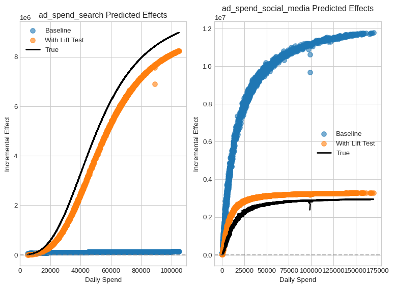
Much better, right? And it was implemented with a really modular and flexible code. You could wrap any effect with LiftExperimentLikelihood to add lift test data to guide its behaviour. Nevertheless, this is not the end of the story.
2.3 Add Attribution Signals with ExactLikelihood
Attribution models can provide daily signals. If available, you can incorporate them by adding another likelihood term via ExactLikelihood.
We create a synthetic attribution signal by multiplying the true effect with a random noise factor.
from prophetverse.effects import ExactLikelihood

rng = np.random.default_rng(42)

# Generate attribution signals for search and social media channels
attr_search = true_components[["ad_spend_search"]] * rng.normal(
    1, 0.1, size=(len(y), 1)
)
attr_social = true_components[["ad_spend_social_media"]] * rng.normal(
    1, 0.1, size=(len(y), 1)
)

# Display the first few rows of the social media attribution signal
attr_social.head()| ad_spend_social_media | |
|---|---|
| 2000-01-01 | 2.171846e+06 |
| 2000-01-02 | 2.625088e+06 |
| 2000-01-03 | 2.983027e+06 |
| 2000-01-04 | 2.836756e+06 |
| 2000-01-05 | 2.520331e+06 |
model_umm = model_lift.clone()
model_umm.set_params(
    exogenous_effects=model_lift.get_params()["exogenous_effects"]
    + [
        (
            "attribution_search",
            ExactLikelihood("ad_spend_search", attr_search, 0.01),
            None,
        ),
        (
            "attribution_social_media",
            ExactLikelihood("ad_spend_social_media", attr_social, 0.01),
            None,
        ),
    ]
)
model_umm.fit(y=y, X=X)
Prophetverse(exogenous_effects=[('yearly_seasonality',
LinearFourierSeasonality(effect_mode='multiplicative',
fourier_terms_list=[5],
freq='D',
prior_scale=0.1,
sp_list=[365.25]),
None),
('weekly_seasonality',
LinearFourierSeasonality(effect_mode='multiplicative',
fourier_terms_list=[3],
freq='D',
prior_scale=0.05,
sp_list=[7]),
None),
('ad_spend_search',
LiftExp...
2000-01-04 2.836756e+06
2000-01-05 2.520331e+06
... ...
2004-12-28 1.012305e+06
2004-12-29 1.108765e+06
2004-12-30 1.070854e+06
2004-12-31 1.027756e+06
2005-01-01 1.012141e+06
[1828 rows x 1 columns]),
None)],
inference_engine=MAPInferenceEngine(num_steps=5000,
optimizer=LBFGSSolver(max_linesearch_steps=300,
memory_size=300)),
trend=PiecewiseLinearTrend(changepoint_interval=100))Please rerun this cell to show the HTML repr or trust the notebook.Prophetverse(exogenous_effects=[('yearly_seasonality',
LinearFourierSeasonality(effect_mode='multiplicative',
fourier_terms_list=[5],
freq='D',
prior_scale=0.1,
sp_list=[365.25]),
None),
('weekly_seasonality',
LinearFourierSeasonality(effect_mode='multiplicative',
fourier_terms_list=[3],
freq='D',
prior_scale=0.05,
sp_list=[7]),
None),
('ad_spend_search',
LiftExp...
2000-01-04 2.836756e+06
2000-01-05 2.520331e+06
... ...
2004-12-28 1.012305e+06
2004-12-29 1.108765e+06
2004-12-30 1.070854e+06
2004-12-31 1.027756e+06
2005-01-01 1.012141e+06
[1828 rows x 1 columns]),
None)],
inference_engine=MAPInferenceEngine(num_steps=5000,
optimizer=LBFGSSolver(max_linesearch_steps=300,
memory_size=300)),
trend=PiecewiseLinearTrend(changepoint_interval=100))PiecewiseLinearTrend(changepoint_interval=100)
LinearFourierSeasonality(effect_mode='multiplicative', fourier_terms_list=[5],
freq='D', prior_scale=0.1, sp_list=[365.25])LinearFourierSeasonality(effect_mode='multiplicative', fourier_terms_list=[3],
freq='D', prior_scale=0.05, sp_list=[7])LiftExperimentLikelihood(effect=ChainedEffects(steps=[('adstock',
GeometricAdstockEffect()),
('saturation',
HillEffect(effect_mode='additive',
half_max_prior=<numpyro.distributions.continuous.HalfNormal object at 0x7f0bbc7b1b10 with batch shape () and event shape ()>,
input_scale=1000000.0,
max_effect_prior=<numpyro.distributions.continuous.HalfNormal object at 0x7f0b...
2001-02-02 1.212479 67857.642170 88071.282712
2001-05-21 1.178636 71337.927880 93445.016948
2003-05-06 0.644814 25609.287364 21843.082411
2000-07-31 1.012828 92617.293678 85766.681515
2002-07-03 1.267595 57443.596207 66595.562035
2004-09-27 1.369890 41546.443755 50176.823146
2000-10-25 0.985062 72757.343228 70195.986606
2002-11-02 0.834577 19043.272758 18373.397899,
prior_scale=0.05)ChainedEffects(steps=[('adstock', GeometricAdstockEffect()),
('saturation',
HillEffect(effect_mode='additive',
           half_max_prior=<numpyro.distributions.continuous.HalfNormal object at 0x7f0bbc7b1b10 with batch shape () and event shape ()>,
           input_scale=1000000.0,
           max_effect_prior=<numpyro.distributions.continuous.HalfNormal object at 0x7f0b90b2c390 with batch shape () and event shape ()>,
slope_prior=<numpyro.distributions.continuous.InverseGamma object at 0x7f0b4c6d3750 with batch shape () and event shape ()>))])GeometricAdstockEffect()
HillEffect(effect_mode='additive',
           half_max_prior=<numpyro.distributions.continuous.HalfNormal object at 0x7f0bbc7b1b10 with batch shape () and event shape ()>,
           input_scale=1000000.0,
           max_effect_prior=<numpyro.distributions.continuous.HalfNormal object at 0x7f0b90b2c390 with batch shape () and event shape ()>,
slope_prior=<numpyro.distributions.continuous.InverseGamma object at 0x7f0b4c6d3750 with batch shape () and event shape ()>)LiftExperimentLikelihood(effect=ChainedEffects(steps=[('adstock',
GeometricAdstockEffect()),
('saturation',
HillEffect(effect_mode='additive',
half_max_prior=<numpyro.distributions.continuous.HalfNormal object at 0x7f0bbc7b1b10 with batch shape () and event shape ()>,
input_scale=1000000.0,
max_effect_prior=<numpyro.distributions.continuous.HalfNormal object at 0x7f0b...
2001-02-02 1.085461 38129.336619 47626.107330
2001-05-21 0.961702 50010.574434 73721.957893
2003-05-06 1.099837 2893.044038 2702.425237
2000-07-31 1.028477 105196.357631 125200.174092
2002-07-03 1.053316 25537.869750 38025.254409
2004-09-27 1.010456 8523.749415 11037.466255
2000-10-25 0.980559 50964.957119 65038.733878
2002-11-02 1.355164 1195.765141 1603.253926,
prior_scale=0.05)ChainedEffects(steps=[('adstock', GeometricAdstockEffect()),
('saturation',
HillEffect(effect_mode='additive',
half_max_prior=<numpyro.distributions.continuous.HalfNormal object at 0x7f0bbc7b1b10 with batch shape () and event shape ()>,
input_scale=1000000.0,
max_effect_prior=<numpyro.distributions.continuous.HalfNormal object at 0x7f0b90b2c390 with batch shape () and event shape ()>,
slope_prior=<numpyro.distributions.continuous.InverseGamma object at 0x7f0b4c6d3750 with batch shape () and event shape ()>))])GeometricAdstockEffect()
HillEffect(effect_mode='additive',
half_max_prior=<numpyro.distributions.continuous.HalfNormal object at 0x7f0bbc7b1b10 with batch shape () and event shape ()>,
input_scale=1000000.0,
max_effect_prior=<numpyro.distributions.continuous.HalfNormal object at 0x7f0b90b2c390 with batch shape () and event shape ()>,
slope_prior=<numpyro.distributions.continuous.InverseGamma object at 0x7f0b4c6d3750 with batch shape () and event shape ()>)ExactLikelihood(effect_name='ad_spend_search', prior_scale=0.01,
reference_df= ad_spend_search
2000-01-01 8.682649e+06
2000-01-02 7.542228e+06
2000-01-03 9.091821e+06
2000-01-04 9.259557e+06
2000-01-05 6.785853e+06
... ...
2004-12-28 3.547301e+06
2004-12-29 2.771639e+06
2004-12-30 2.972279e+06
2004-12-31 3.226681e+06
2005-01-01 3.605501e+06
[1828 rows x 1 columns])ExactLikelihood(effect_name='ad_spend_social_media', prior_scale=0.01,
reference_df= ad_spend_social_media
2000-01-01 2.171846e+06
2000-01-02 2.625088e+06
2000-01-03 2.983027e+06
2000-01-04 2.836756e+06
2000-01-05 2.520331e+06
... ...
2004-12-28 1.012305e+06
2004-12-29 1.108765e+06
2004-12-30 1.070854e+06
2004-12-31 1.027756e+06
2005-01-01 1.012141e+06
[1828 rows x 1 columns])MAPInferenceEngine(num_steps=5000,
optimizer=LBFGSSolver(max_linesearch_steps=300,
memory_size=300))components_umm = model_umm.predict_components(X=X, fh=X.index)
fig, axs = plt.subplots(2, 1, figsize=(8, 10), sharex=True)
for ax, channel in zip(axs, ["ad_spend_search", "ad_spend_social_media"]):
ax.scatter(X[channel], y_pred_components[channel], label="Baseline", alpha=0.4)
ax.scatter(X[channel], components_lift[channel], label="With Lift Test", alpha=0.4)
ax.scatter(X[channel], components_umm[channel], label="With Attribution", alpha=0.4)
ax.plot(X[channel], true_components[channel], label="True Effect", color="black")
ax.set_title(channel)
ax.legend()
plt.tight_layout()
plt.show()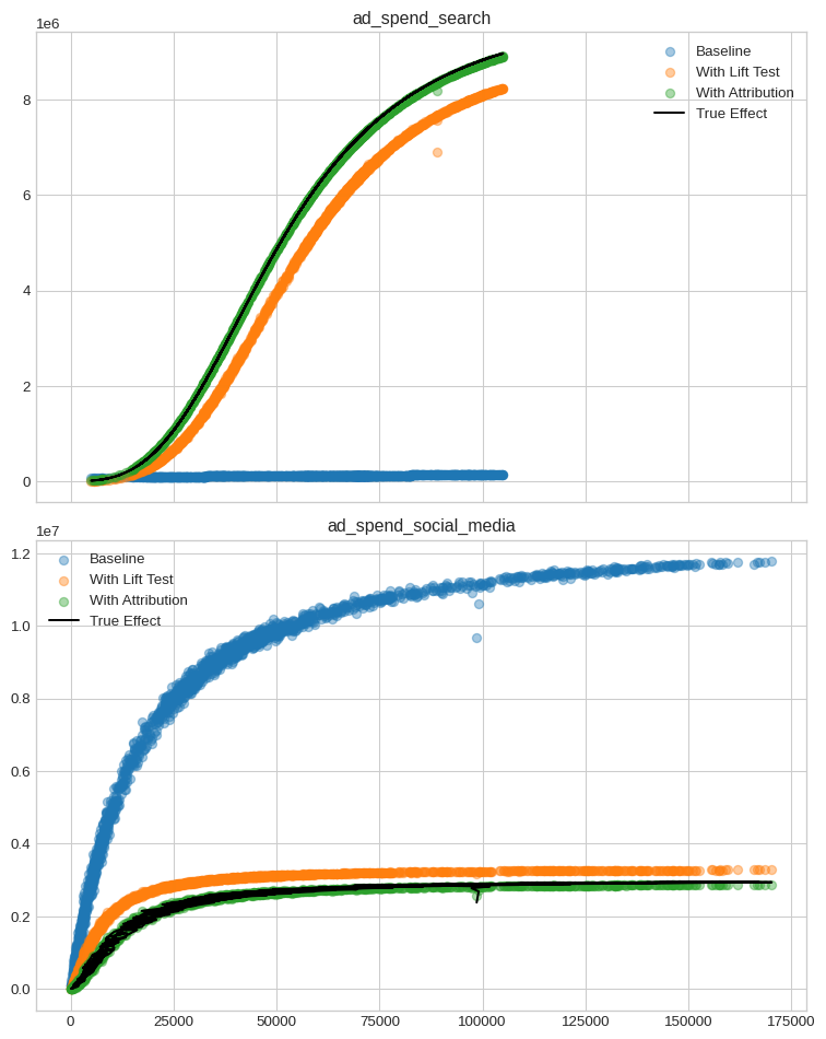
Even better! And, due to sktime-like interface, wrapping and adding new effects is easy.
Final Thoughts: Toward Unified Marketing Measurement
✅ What we learned:
1. Adstock + saturation are essential to capture media dynamics.
2. Good predictions ≠ good attribution.
3. Causal data like lift tests can correct misattribution.
4. Attribution signals add further constraints.
🛠️ Use this when:
* Channels are correlated → Use lift tests.
* You have granular model output → Add attribution likelihoods.
🧪 Model selection tip:
Always validate causal logic, not just fit quality.
With Prophetverse, you can combine observational, experimental, and model-based signals into one coherent MMM+UMM pipeline.