Budget Optimization for Single and Multiple Time Series

Use Prophetverse to optimize media budget allocation across channels for one or many time series.

In this tutorial, you’ll learn how to use Prophetverse’s budget-optimization module to:

Allocate daily spend across channels to maximize a key performance indicator (KPI).
Minimize total spend required to achieve a target KPI.
Handle both single and multiple time series (e.g., different geographies) seamlessly.

You’ll also see how to switch between different parametrizations without hassle, such as:

Daily-spend mode: Optimize the exact dollar amount for each day and channel.
Share-of-budget mode: Fix your overall spending pattern and optimize only the channel shares.

By the end, you’ll know how to pick the right setup for your campaign goals and make adjustments in seconds.

Part 1: Optimizing for a Single Time Series

1.1. Setting Up the Problem

First, let’s set up our environment and load the data for a single time series optimization.

import numpyro

numpyro.enable_x64()

import matplotlib.pyplot as plt
import matplotlib.dates as mdates
import pandas as pd

plt.style.use("seaborn-v0_8-whitegrid")

1.1.1. Load synthetic data

We will load a synthetic dataset and a pre-fitted Prophetverse model.

from prophetverse.datasets._mmm.dataset1 import get_dataset

y, X, lift_tests, true_components, model = get_dataset()

1.1.2. Utility plotting functions

This helper function will allow us to compare spend before and after optimization.

Code

def plot_spend_comparison(
    X_baseline,
    X_optimized,
    channels,
    indexer,
    *,
    baseline_title="Baseline Spend: Pre-Optimization",
    optimized_title="Optimized Spend: Maximizing KPI",
    figsize=(8, 4),
):
    fig, ax = plt.subplots(1, 2, figsize=figsize)

    X_baseline.loc[indexer, channels].plot(ax=ax[0], linewidth=2)
    X_optimized.loc[indexer, channels].plot(ax=ax[1], linewidth=2, linestyle="--")

    ax[0].set_title(baseline_title, fontsize=14, weight="bold")
    ax[1].set_title(optimized_title, fontsize=14, weight="bold")

    for a in ax:
        a.set_ylabel("Spend")
        a.set_xlabel("Date")
        a.legend(loc="upper right", frameon=True)
        a.grid(axis="x", visible=False)
        a.grid(axis="y", linestyle="--", alpha=0.7)
        a.xaxis.set_major_formatter(mdates.DateFormatter("%b"))

    # Align y-axis
    y_max = max(
        X_baseline.loc[indexer, channels].max().max(),
        X_optimized.loc[indexer, channels].max().max(),
    )
    for a in ax:
        a.set_ylim(0, y_max * 1.05)

    plt.tight_layout()
    return fig, ax

1.2. Budget Optimization

The budget-optimization module is composed of three main components:

The objective function: What you want to optimize (e.g., maximize KPI).
The constraints: Rules the optimization must follow (e.g., total budget).
The parametrization transform: How the problem is parametrized (e.g., daily spend vs. channel shares).

1.2.1. Maximizing a KPI

The BudgetOptimizer class is the main entry point. By default, it optimizes the daily spend for each channel to maximize a given KPI.

from prophetverse.budget_optimization import (
    BudgetOptimizer,
    TotalBudgetConstraint,
    MaximizeKPI,
)

budget_optimizer = BudgetOptimizer(
    objective=MaximizeKPI(),
    constraints=[TotalBudgetConstraint()],
    options={"disp": True, "maxiter":1000},
)

Let’s define our optimization horizon:

horizon = pd.period_range("2004-12-01", "2004-12-31", freq="D")

Now, we run the optimization:

import time

start_time = time.time()
X_opt = budget_optimizer.optimize(
    model=model,
    X=X,
    horizon=horizon,
    columns=["ad_spend_search", "ad_spend_social_media"],
)
optimization_time = time.time() - start_time
print(f"Optimization completed in {optimization_time:.2f} seconds")

Optimization terminated successfully    (Exit mode 0)
            Current function value: -754679704.6820625
            Iterations: 108
            Function evaluations: 125
            Gradient evaluations: 104
Optimization completed in 2.71 seconds

Baseline vs. optimized spend

Let’s compare the model’s predictions before and after the optimization.

y_pred_baseline = model.predict(X=X, fh=horizon)
y_pred_opt = model.predict(X=X_opt, fh=horizon)

fig, ax = plot_spend_comparison(
    X,
    X_opt,
    ["ad_spend_search", "ad_spend_social_media"],
    horizon,
)

kpi_gain = y_pred_opt.sum() / y_pred_baseline.sum() - 1
fig.suptitle(f"KPI gain: +{kpi_gain:.2%}", fontsize=16,weight="bold", y=1.02)
fig.tight_layout()
fig.show()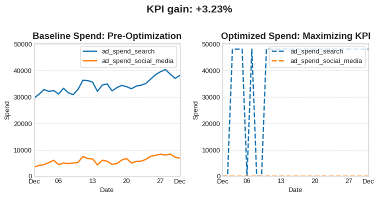

1.2.2. Reparametrization: Optimizing channel share

Instead of daily spend, we can optimize the share of the budget for each channel. This is useful for keeping a fixed spending pattern (e.g., for seasonal campaigns).

from prophetverse.budget_optimization import InvestmentPerChannelTransform

budget_optimizer_reparam = BudgetOptimizer(
    objective=MaximizeKPI(),
    constraints=[TotalBudgetConstraint()],
    parametrization_transform=InvestmentPerChannelTransform(),
    options={"disp": True},
)

X_opt_reparam = budget_optimizer_reparam.optimize(
    model=model,
    X=X,
    horizon=horizon,
    columns=["ad_spend_search", "ad_spend_social_media"],
)

Optimization terminated successfully    (Exit mode 0)
            Current function value: -738733788.63574
            Iterations: 13
            Function evaluations: 42
            Gradient evaluations: 12

Baseline vs. optimized spend

y_pred_opt_reparam = model.predict(X=X_opt_reparam, fh=horizon)

fig, ax = plot_spend_comparison(
    X,
    X_opt_reparam,
    ["ad_spend_search", "ad_spend_social_media"],
    horizon,
)

kpi_gain = y_pred_opt_reparam.sum() / y_pred_baseline.sum() - 1
fig.suptitle(f"KPI gain: +{kpi_gain:.2%}", fontsize=16, weight="bold", y=1.02)
fig.tight_layout()
fig.show()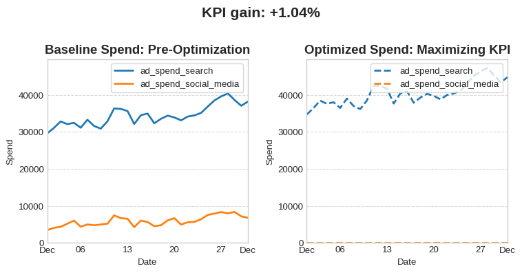

1.2.3. Minimizing budget to reach a target

We can also change the objective to find the minimum investment required to achieve a specific KPI target. Let’s say we want a 30% increase in KPI compared to 2003.

from prophetverse.budget_optimization import (
    MinimizeBudget,
    MinimumTargetResponse,
)

target = y.loc["2003-12"].sum() * 1.30

budget_optimizer_min = BudgetOptimizer(
    objective=MinimizeBudget(),
    constraints=[MinimumTargetResponse(target_response=target, constraint_type="eq")],
    options={"disp": True, "maxiter" : 300},
)

X0 = X.copy()
X_opt_min = budget_optimizer_min.optimize(
    model=model,
    X=X0,
    horizon=horizon,
    columns=["ad_spend_search", "ad_spend_social_media"],
)

Optimization terminated successfully    (Exit mode 0)
            Current function value: 3796555.321062599
            Iterations: 201
            Function evaluations: 204
            Gradient evaluations: 201

Budget and prediction comparison

plot_spend_comparison(
    X0,
    X_opt_min,
    ["ad_spend_search", "ad_spend_social_media"],
    indexer=horizon,
)
plt.show()

y_pred_baseline_min = model.predict(X=X0, fh=horizon)
y_pred_opt_min = model.predict(X=X_opt_min, fh=horizon)

print(
    f"MMM Predictions \n",
    f"Baseline KPI: {y_pred_baseline_min.sum()/1e9:.2f} B \n",
    f"Optimized KPI: {y_pred_opt_min.sum()/1e9:.2f} B \n",
    f"Target KPI: {target/1e9:.2f} B \n",
    "Baseline spend: ",
    X0.loc[horizon, ["ad_spend_search", "ad_spend_social_media"]].sum().sum(),
    "\n",
    "Optimized spend: ",
    X_opt_min.loc[horizon, ["ad_spend_search", "ad_spend_social_media"]].sum().sum(),
    "\n",
)

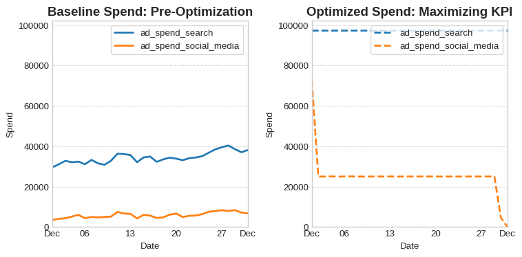
MMM Predictions 
 Baseline KPI: 0.73 B 
 Optimized KPI: 0.97 B 
 Target KPI: 0.97 B 
 Baseline spend:  1250679.3427392421 
 Optimized spend:  3796555.3210625993

Part 2: Optimizing for Multiple Time Series (Panel Data)

The same BudgetOptimizer can be used for multiple time series (e.g., different geographies) without any changes to the API.

2.1. Setting Up the Problem for Panel Data

The main difference is that for panel data, we use a multi-index DataFrame, following sktime conventions.

2.1.1. Load synthetic panel data

from prophetverse.datasets._mmm.dataset1_panel import get_dataset

y_panel, X_panel, lift_tests_panel, true_components_panel, fitted_model_panel = get_dataset()

y_panel

		0
group	date
a	2000-01-01	1.120218e+07
	2000-01-02	1.146048e+07
	2000-01-03	1.156324e+07
	2000-01-04	1.161396e+07
	2000-01-05	1.162758e+07
...	...	...
b	2004-12-28	2.473478e+07
	2004-12-29	2.718986e+07
	2004-12-30	2.554932e+07
	2004-12-31	2.343510e+07
	2005-01-01	2.078426e+07

3656 rows × 1 columns

2.1.2. Utility plotting functions for panel data

We’ll define a new plotting function to handle the multi-indexed data.

Code

def plot_spend_comparison_panel(
    X_baseline,
    X_optimized,
    channels,
    indexer,
    *,
    baseline_title="Baseline Spend: Pre-Optimization",
    optimized_title="Optimized Spend: Maximizing KPI",
    figsize=(8, 4),
):
    series_idx = X_baseline.index.droplevel(-1).unique().tolist()
    fig, axs = plt.subplots(len(series_idx), 2, figsize=figsize, squeeze=False)

    for i, series in enumerate(series_idx):
        _X_baseline = X_baseline.loc[series]
        _X_optimized = X_optimized.loc[series]
        ax_row = axs[i]
        _X_baseline.loc[indexer, channels].plot(ax=ax_row[0], linewidth=2)
        _X_optimized.loc[indexer, channels].plot(
            ax=ax_row[1], linewidth=2, linestyle="--"
        )

        ax_row[0].set_title(f"{series}: {baseline_title}", fontsize=14, weight="bold")
        ax_row[1].set_title(f"{series}: {optimized_title}", fontsize=14, weight="bold")

        for a in ax_row:
            a.set_ylabel("Spend")
            a.set_xlabel("Date")
            a.legend(loc="upper right", frameon=True)
            a.grid(axis="x", visible=False)
            a.grid(axis="y", linestyle="--", alpha=0.7)
            a.xaxis.set_major_formatter(mdates.DateFormatter("%b"))

        y_max = max(
            _X_baseline.loc[indexer, channels].max().max(),
            _X_optimized.loc[indexer, channels].max().max(),
        )
        for a in ax_row:
            a.set_ylim(0, y_max * 1.05)

    plt.tight_layout()
    return fig, axs

2.2. Budget Optimization for Panel Data

2.2.1. Maximizing a KPI

By default, BudgetOptimizer will optimize the daily spend for each channel for each series.

budget_optimizer_panel = BudgetOptimizer(
    objective=MaximizeKPI(),
    constraints=[TotalBudgetConstraint()],
    options={"disp": True, "maxiter": 1000},
)

X_opt_panel = budget_optimizer_panel.optimize(
    model=fitted_model_panel,
    X=X_panel,
    horizon=horizon,
    columns=["ad_spend_search", "ad_spend_social_media"],
)

Optimization terminated successfully    (Exit mode 0)
            Current function value: -1723014730.7615
            Iterations: 198
            Function evaluations: 198
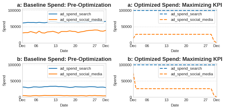
            Gradient evaluations: 197

Baseline vs. optimized spend

y_pred_baseline_panel = fitted_model_panel.predict(X=X_panel, fh=horizon)
y_pred_opt_panel = fitted_model_panel.predict(X=X_opt_panel, fh=horizon)

fig, ax = plot_spend_comparison_panel(
    X_panel,
    X_opt_panel,
    ["ad_spend_search", "ad_spend_social_media"],
    horizon,
)

kpi_gain = y_pred_opt_panel.values.sum() / y_pred_baseline_panel.values.sum() - 1
fig.suptitle(f"Total KPI gain: +{kpi_gain:.2%}", fontsize=16, weight="bold", y=1.03)
fig.tight_layout()
fig.show()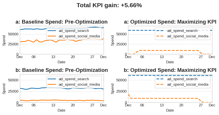

2.2.2. Reparametrization for Panel Data

With panel data, we have more reparametrization options.

Optimizing channel share (globally)

This optimizes the share of budget for each channel, keeping the total investment and spending pattern fixed. The channel shares are the same across all series.

from prophetverse.budget_optimization import InvestmentPerChannelTransform

budget_optimizer_panel_ch = BudgetOptimizer(
    objective=MaximizeKPI(),
    constraints=[TotalBudgetConstraint()],
    parametrization_transform=InvestmentPerChannelTransform(),
    options={"disp": True},
)

X_opt_panel_ch = budget_optimizer_panel_ch.optimize(
    model=fitted_model_panel,
    X=X_panel,
    horizon=horizon,
    columns=["ad_spend_search", "ad_spend_social_media"],
)
# You can plot the results using plot_spend_comparison_panel

Optimization terminated successfully    (Exit mode 0)
            Current function value: -1674672737.6774194
            Iterations: 13
            Function evaluations: 13
            Gradient evaluations: 13

Optimizing investment per series

This keeps the channel shares fixed within each series but optimizes the allocation of the total budget across the different series.

from prophetverse.budget_optimization.parametrization_transformations import InvestmentPerSeries

budget_optimizer_panel_s = BudgetOptimizer(
    objective=MaximizeKPI(),
    constraints=[TotalBudgetConstraint()],
    parametrization_transform=InvestmentPerSeries(),
    options={"disp": True},
)

X_opt_panel_s = budget_optimizer_panel_s.optimize(
    model=fitted_model_panel,
    X=X_panel,
    horizon=horizon,
    columns=["ad_spend_search", "ad_spend_social_media"],
)
# You can plot the results using plot_spend_comparison_panel

Optimization terminated successfully    (Exit mode 0)
            Current function value: -1680449341.6035411
            Iterations: 13
            Function evaluations: 13
            Gradient evaluations: 13

Optimizing share per channel and series

This is the most granular reparametrization, optimizing the share of budget for each channel within each series.

from prophetverse.budget_optimization.parametrization_transformations import InvestmentPerChannelAndSeries

budget_optimizer_panel_cs = BudgetOptimizer(
    objective=MaximizeKPI(),
    constraints=[TotalBudgetConstraint()],
    parametrization_transform=InvestmentPerChannelAndSeries(),
    options={"disp": True},
)

X_opt_panel_cs = budget_optimizer_panel_cs.optimize(
    model=fitted_model_panel,
    X=X_panel,
    horizon=horizon,
    columns=["ad_spend_search", "ad_spend_social_media"],
)
# You can plot the results using plot_spend_comparison_panel

Optimization terminated successfully    (Exit mode 0)
            Current function value: -1717879098.7472155
            Iterations: 29
            Function evaluations: 38
            Gradient evaluations: 28

2.2.3. Minimizing budget to reach a target with Panel Data

Let’s find the minimum budget to achieve a 20% KPI increase across all series.

target_panel = y_panel.loc[pd.IndexSlice[:, horizon],].values.sum() * 1.2

budget_optimizer_min_panel = BudgetOptimizer(
    objective=MinimizeBudget(),
    constraints=[MinimumTargetResponse(target_response=target_panel, constraint_type="eq")],
    options={"disp": True, "maxiter": 300},
)

X0_panel = X_panel.copy()
X_opt_min_panel = budget_optimizer_min_panel.optimize(
    model=fitted_model_panel,
    X=X0_panel,
    horizon=horizon,
    columns=["ad_spend_search", "ad_spend_social_media"],
)

Optimization terminated successfully    (Exit mode 0)
            Current function value: 7755666.679734466
            Iterations: 285
            Function evaluations: 287
            Gradient evaluations: 285

Budget and prediction comparison

plot_spend_comparison_panel(
    X0_panel,
    X_opt_min_panel,
    ["ad_spend_search", "ad_spend_social_media"],
    indexer=horizon,
)
plt.show()

y_pred_baseline_min_panel = fitted_model_panel.predict(X=X0_panel, fh=horizon)
y_pred_opt_min_panel = fitted_model_panel.predict(X=X_opt_min_panel, fh=horizon)

print(
    f"MMM Predictions \n",
    f"Baseline KPI: {y_pred_baseline_min_panel.values.sum()/1e9:.2f} B \n",
    f"Optimized KPI: {y_pred_opt_min_panel.values.sum()/1e9:.2f} B \n",
    f"Target KPI: {target_panel/1e9:.2f} B \n",
    "Baseline spend: ",
    X0_panel.loc[
        pd.IndexSlice[:, horizon], ["ad_spend_search", "ad_spend_social_media"]
    ]
    .sum()
    .sum(),
    "\n",
    "Optimized spend: ",
    X_opt_min_panel.loc[
        pd.IndexSlice[:, horizon], ["ad_spend_search", "ad_spend_social_media"]
    ]
    .sum()
    .sum(),
    "\n",
)

MMM Predictions 
 Baseline KPI: 1.63 B 
 Optimized KPI: 1.96 B 
 Target KPI: 1.96 B 
 Baseline spend:  4179163.3068621266 
 Optimized spend:  7755666.679734467

Conclusion

We have seen the capabilities of the budget-optimization module for both single and multiple time series. The three key components are the objective function, the constraints, and the parametrization transform. You can also create your own custom components to tailor the optimization to your specific needs.