This how‑to shows how to use the Beta likelihood for a proportion / percentage target using the same sktime-style API demonstrated in other tutorials.
Why Beta? Because the target is naturally bounded in (0,1), and Beta likelihood can provide probabilistic intervals in (0,1). The likelihood="beta" option internally applies a link that guarantees valid predictions.
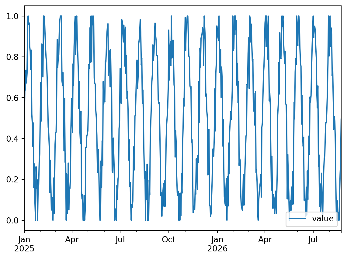
1. Load data and build a (0,1) target
import numpy as npimport pandas as pdfrom sktime.split import temporal_train_test_split= 1000 = pd.DataFrame(= {"value" : np.sin(np.arange(num_obs)* 2 * np.pi/ 30 )* 0.45 + 0.5 },= pd.period_range("2025-01-01" ,= num_obs,= "D" ,+= np.random.normal(0 , 0.1 , size= y.shape)= y.clip(1e-6 , 1 - 1e-6 )= temporal_train_test_split(y, test_size= 0.4 )
2. Specify model components
We use a piecewise linear trend plus weekly and yearly seasonality. The API mirrors the univariate tutorial: pass trend=..., supply exogenous_effects as a list of tuples, and choose likelihood="beta".
import numpyrofrom prophetverse.effects.trend import PiecewiseLinearTrendfrom prophetverse.effects.fourier import LinearFourierSeasonalityfrom prophetverse.effects.target.univariate import BetaTargetLikelihoodfrom prophetverse.utils import no_input_columnsfrom prophetverse.engine import MAPInferenceEnginefrom prophetverse.sktime import Prophetverse= ("seasonality" ,= "D" ,= [30 ], # weekly + yearly = [30 ],= 1 ,= "additive" ,= Prophetverse(= "flat" ,= [seasonality],= BetaTargetLikelihood(noise_scale= 0.2 ), # <— key change = MAPInferenceEngine(),= 1 ,= y_train)
/opt/hostedtoolcache/Python/3.11.15/x64/lib/python3.11/site-packages/tqdm/auto.py:21: TqdmWarning: IProgress not found. Please update jupyter and ipywidgets. See https://ipywidgets.readthedocs.io/en/stable/user_install.html
  from .autonotebook import tqdm as notebook_tqdm
Prophetverse(exogenous_effects=[('seasonality',
                                 LinearFourierSeasonality(fourier_terms_list=[30],
                                                          freq='D',
                                                          prior_scale=1,
                                                          sp_list=[30]),
                                 '^$')],
             inference_engine=MAPInferenceEngine(),
             likelihood=BetaTargetLikelihood(noise_scale=0.2), scale=1,
             trend='flat')
Please rerun this cell to show the HTML repr or trust the notebook.
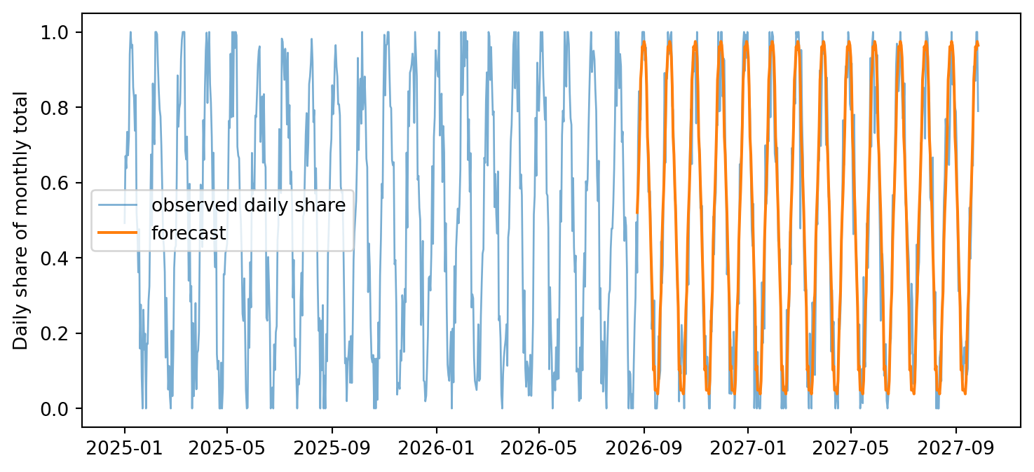
3. Forecast the next 180 days
import pandas as pd= y_test.index= model.predict(fh= fh)
2026-08-24
0.485824
2026-08-25
0.561676
2026-08-26
0.639714
2026-08-27
0.727727
2026-08-28
0.904001
4. Plot
import matplotlib.pyplot as plt= plt.subplots(figsize= (9 , 4 ))= "observed daily share" , lw= 1 , alpha= 0.6 = "forecast" , color= "C1" )"Daily share of monthly total" )
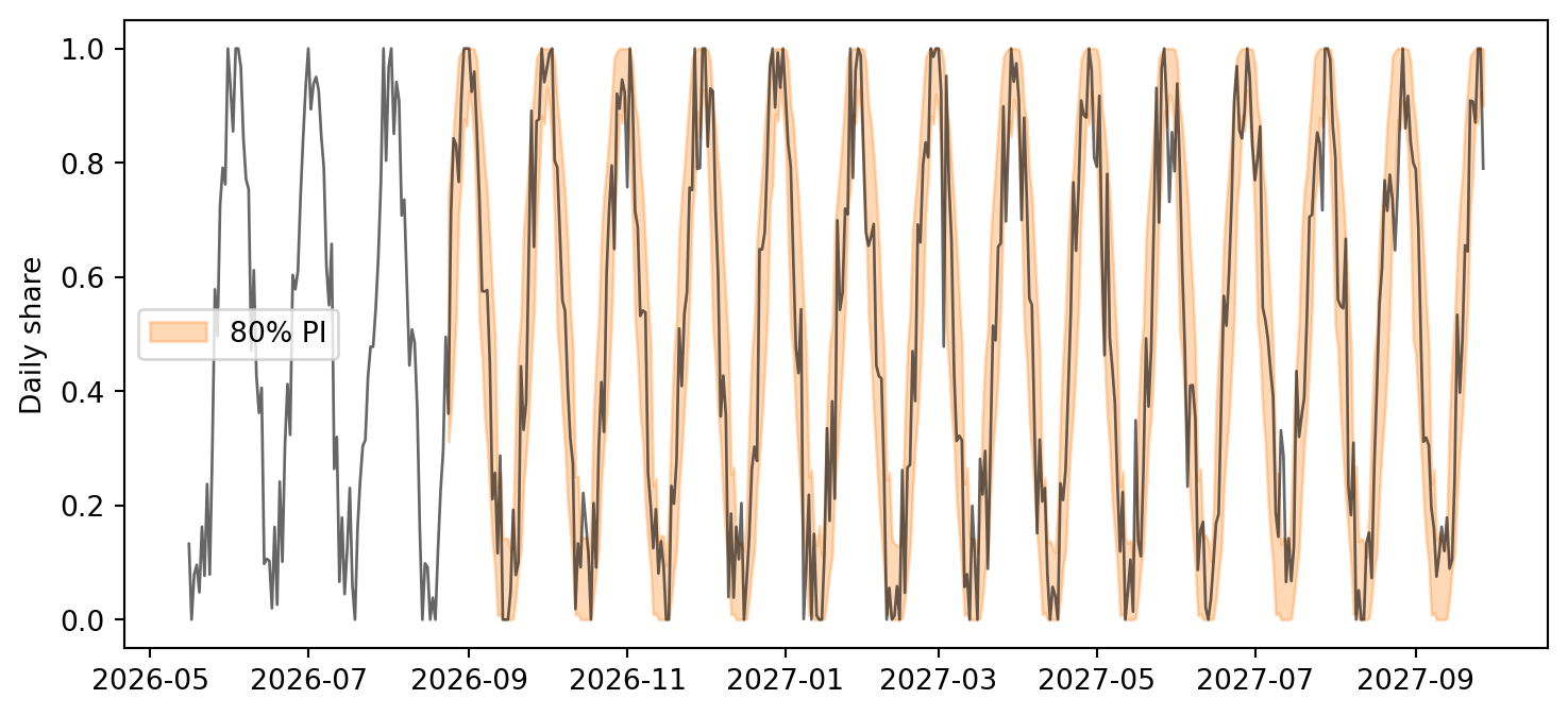
5. Probabilistic forecast (quantiles)
= model.predict_quantiles(fh= fh, alpha= [0.1 , 0.9 ])= plt.subplots(figsize= (9 , 4 ))0 ],- 1 ],= "C1" ,= 0.3 ,= "80% PI" ,- (len (fh) + 100 ):].index.to_timestamp(), y.iloc[- (len (fh) + 100 ):], lw= 1 , alpha= 0.6 , color= "k" )"Daily share" )
Notes & Tips
Ensure the target is strictly inside (0,1), excluding the boundaries.
noise_scale controls dispersion of the Beta (smaller => tighter intervals).The same pattern works for conversion rates, CTR, retention proportions, etc.
Switch to full Bayesian inference by setting inference_engine=MCMCInferenceEngine(...) if you need richer uncertainty.