Basics of Prophetverse API

Prophetverse is a powerful tool for building customized and glass-box forecasting and mix models. In Prophetverse, we define each component of the model as a separate effect, making this library extremely flexible to attend your specific needs.

In this page, we will:

Understand the structure of y (the target) and X (media & control variables) using the sktime interface.
Understand the hyperparameters of Prophetverse
Fit your first Bayesian MMM and generate forecasts.

1. Data Structures (`y` and `X`)

Prophetverse uses the sktime forecasting API. The essentials:

y: a pandas DataFrame indexed by a time index (pd.DatetimeIndex or pd.PeriodIndex). Single column for univariate MMM (e.g. revenue):

	revenue
2020-01-01	0.539791
2020-01-02	0.386945
2020-01-03	0.846947
2020-01-04	0.868224
2020-01-05	0.000316

For panel datasets (e.g. in the case of multiple products or regions), use a MultiIndex, where the first index level is the entity (e.g. product or region) and the second level is the time.

		revenue
product
product_a	2020-01-01	0.941121
	2020-01-02	0.087908
	2020-01-03	0.271994
	2020-01-04	0.859156
	2020-01-05	0.851053
...	...	...
product_c	2020-12-27	0.542822
	2020-12-28	0.405629
	2020-12-29	0.159127
	2020-12-30	0.788819
	2020-12-31	0.252980

1098 rows × 1 columns

X: a pandas DataFrame aligned on the same index containing exogenous variables (media spend, price, promotions, macro, etc.). Columns are arbitrary names.

The index type should always be the same for y and X, and every dataframe you use. After choosing Datetime or Period index for y, use the same type for X.

Example of dataset

Here we load a synthetic dataset:

from prophetverse.datasets._mmm.dataset1 import get_dataset

(y, X, *_) = get_dataset()


y.head()

/opt/hostedtoolcache/Python/3.11.13/x64/lib/python3.11/site-packages/tqdm/auto.py:21: TqdmWarning: IProgress not found. Please update jupyter and ipywidgets. See https://ipywidgets.readthedocs.io/en/stable/user_install.html
  from .autonotebook import tqdm as notebook_tqdm

2000-01-01    10815512.0
2000-01-02    11120677.0
2000-01-03    11260387.0
2000-01-04    11322533.0
2000-01-05    11321180.0
Freq: D, dtype: float32

The X looks like this:

X.head()

	ad_spend_search	ad_spend_social_media
2000-01-01	89076.191178	98587.488958
2000-01-02	88891.993106	99066.321168
2000-01-03	89784.955064	97334.106903
2000-01-04	89931.220681	101747.300585
2000-01-05	89184.319596	93825.221809

We will split the dataset into training and testing sets.

from sktime.split import temporal_train_test_split

y_train, y_test, X_train, X_test = temporal_train_test_split(y, X, test_size=0.2)

2. Prophetverse model

Think of Prophetverse as the conerstone of you MMM model. It is a flexible class that allows you to define the trend, seasonality, and custom exogenous effects of your model.

Simple Prophetverse model

We can use a simple Prophetverse model with Linear effects and a seasonality component:

from prophetverse import Prophetverse, LinearEffect, LinearFourierSeasonality

from prophetverse.utils.regex import starts_with, no_input_columns


seasonality_effect = LinearFourierSeasonality(
    sp_list=[365.25, 7],
    fourier_terms_list=[10, 3],
    prior_scale=0.1,
    freq="D",
    effect_mode="additive",
)

ad_spend_effect = LinearEffect()

model = Prophetverse(
    exogenous_effects=[
        ("ad_spend", ad_spend_effect, starts_with("ad")),
        ("seasonality", seasonality_effect, no_input_columns),
    ],
)

model.fit(y=y_train, X=X_train)

Prophetverse(exogenous_effects=[('ad_spend', LinearEffect(), '^(?:ad)'),
                                ('seasonality',
                                 LinearFourierSeasonality(fourier_terms_list=[10,
                                                                              3],
                                                          freq='D',
                                                          prior_scale=0.1,
                                                          sp_list=[365.25, 7]),
                                 '^$')])

Please rerun this cell to show the HTML repr or trust the notebook.

By default, the model will run a MCMC inference to obtain the parameters. We can, however, easily switch to a MAP inference by setting inference_engine=MAPInferenceEngine() in the model constructor. The MAP inference is generally faster but provides point estimates of the parameters.

To run in-sample and out-of-sample forecasts of total revenue, we can simply call predict. We need to pass a “forecasting horizon” (fh) object, that should preferably be an index of the type of our y and X’s index. Since we want to forecast for both train and test timepoints, we use y.index as fh, and pass the full X as exogenous variables.

fh = y.index

y_pred = model.predict(fh=fh, X=X)

y_pred

2000-01-01    14511778.0
2000-01-02    14377447.0
2000-01-03    14452430.0
2000-01-04    14251792.0
2000-01-05    14395013.0
                 ...    
2004-12-28    32311316.0
2004-12-29    32069892.0
2004-12-30    31963730.0
2004-12-31    32207748.0
2005-01-01    32308128.0
Freq: D, Length: 1828, dtype: float32

import matplotlib.pyplot as plt


def plot_forecasts(y_pred):
    fig, ax = plt.subplots(figsize=(10,5))

    ax.plot(y.index.to_timestamp(), y)
    ax.plot(y_pred.index, y_pred)
    ax.axvline(y_train.index.max().to_timestamp(), color="black", linestyle="--", label="Train/Test split")
    fig.show()

plot_forecasts(y_pred)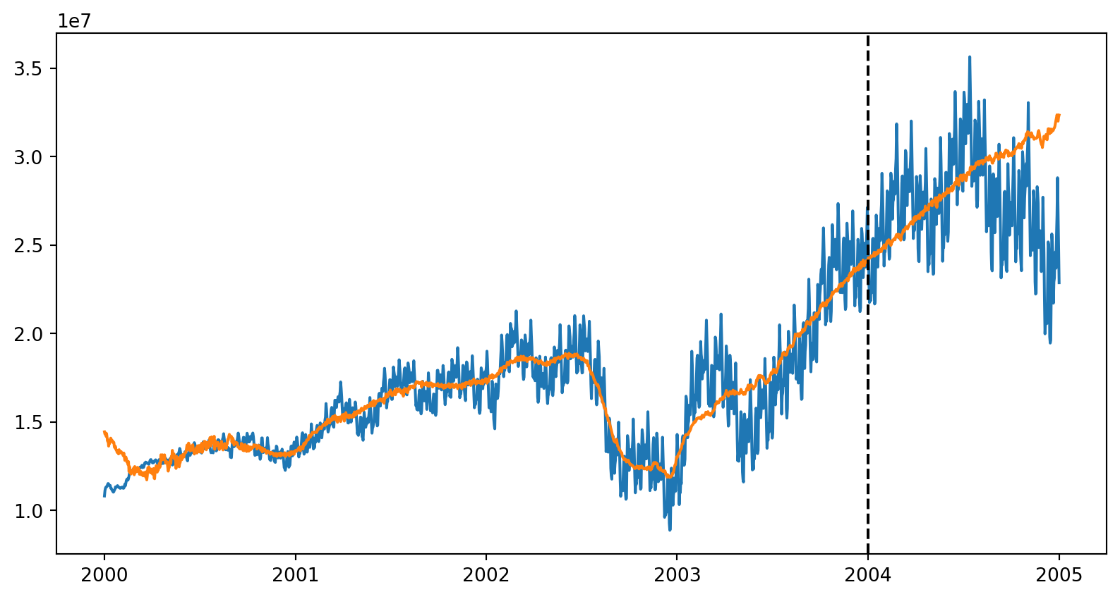

Getting the components

To obtain the contribution of each component, you can use the predict_components method:

components = model.predict_components(fh=fh, X=X)
components.head()

	ad_spend	mean	obs	seasonality	trend
2000-01-01	1981369.125	14511778.0	14529062.0	-1219.737671	12531630.0
2000-01-02	1947268.500	14377447.0	14293655.0	-52385.074219	12482567.0
2000-01-03	2046009.250	14452430.0	14486543.0	-27080.095703	12433500.0
2000-01-04	1905338.875	14251792.0	14198645.0	-37978.394531	12384432.0
2000-01-05	2106310.750	14395013.0	14363289.0	-46668.078125	12335369.0

If you want to obtain all the sample to compute, for example, probabilistic intervals and measure the risk, you can use the predict_component_samples method:

samples = model.predict_component_samples(fh=fh, X=X)
samples

		ad_spend	mean	obs	seasonality	trend
sample
0	2000-01-01	1254598.500	13776006.0	12404012.0	-19438.560547	12540847.0
	2000-01-02	1230125.625	13728084.0	13289906.0	-24919.484375	12522878.0
	2000-01-03	1320823.250	13806783.0	12583303.0	-18948.203125	12504908.0
	2000-01-04	1196263.750	13666452.0	14624822.0	-16750.462891	12486939.0
	2000-01-05	1391929.125	13847936.0	12907703.0	-12964.346680	12468970.0
...	...	...	...	...	...	...
999	2004-12-28	5246423.500	31560616.0	30783596.0	-20673.238281	26334866.0
	2004-12-29	4964901.500	31274182.0	31851820.0	-44955.566406	26354236.0
	2004-12-30	4830923.000	31137578.0	31710976.0	-66945.757812	26373602.0
	2004-12-31	5028303.500	31400522.0	31078702.0	-20773.695312	26392994.0
	2005-01-01	5102370.000	31495128.0	33377402.0	-19621.417969	26412376.0

1828000 rows × 5 columns

1. Data Structures (y and X)

Example of dataset

2. Prophetverse model

Simple Prophetverse model

Getting the components

1. Data Structures (`y` and `X`)