Awareness: Latent and Proxy Variables

Using proxy variables to model latent effects, such as awareness

What you will learn:

Understand how to model latent variables with Prophetverse
Learn how to use proxy variables to improve model accuracy
Model the last-click effect as proportional to awareness, our latent variable.

Latent variables

Tip

From Prophetverse v0.10.0 onwards, we have included a latent variable feature. You only need to add “latent/” as a prefix to the effect name, and it will not be considered as a final component in the additive decomposition. Instead, it can be used as an input to other effects or linked to proxy variables.

In Marketing Mix Modeling, we often encounter latent variables that are not directly observable but significantly influence sales. A common example is brand awareness. It can befined as :

The ability of a potential buyer to recognize or recall that a brand is a member of a certain product category.

Keller, K. L. (1993). Conceptualizing, Measuring, and Managing Customer-Based Brand Equity.

which is clearly affected by marketing activities, and in turn affects sales. Standard MMM approaches may struggle to accurately capture the impact of such latent variables, leading to biased estimates and suboptimal decision-making.

Since we cannot observe these variables directly, it can be hard to model them. However, we propose in Prophetverse the usage of proxy variables that are correlated with the latent variable of interest to help us infer its true causal effect. For example, we might use survey data on brand recognition or social media engagement metrics as proxies for brand awareness and use it as a soft calibration signal.

The idea is simple, but powerful. More formally, if \(Z(t)\) is a latent variable representing brand awareness at time \(t\), and \(P(t)\) is a proxy variable correlated with \(Z(t)\), we can add a new likelihood term:

\[ P(t) \sim \mathcal{N}(\beta Z(t), \sigma^2) \]

For a \(\beta\) with user-defined prior, and \(\sigma^2\) representing the uncertainty in the proxy relationship. If there exists a \(\beta\), then the proxy variable provides additional information about the latent variable, helping to better identify its effect on sales.

1. Dataset

1.1. Loading the data

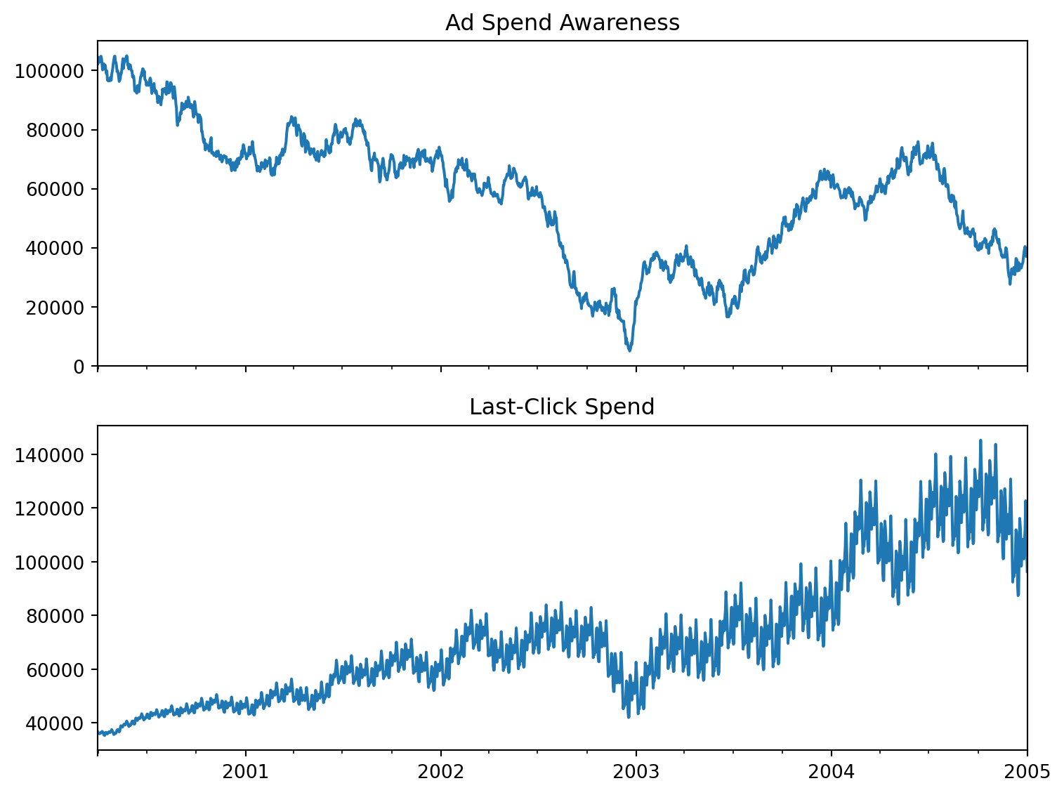
We use a synthetic dataset that simulates a marketing scenario with 2 types of investments:

Investments with impact on brand awareness (e.g., upper-funnel channels like TV, Display, Social Media)
Investments with last-click impact (e.g., Search, Affiliates)

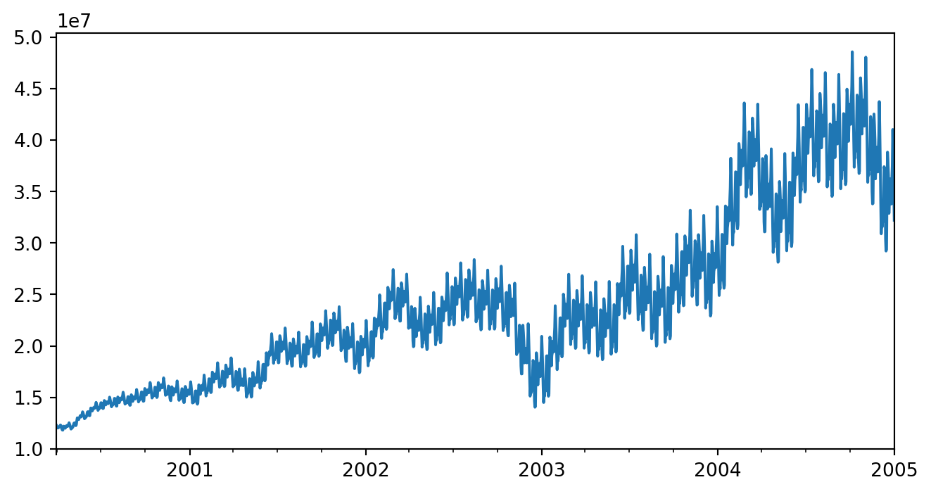
import numpy as np
import matplotlib.pyplot as plt
from prophetverse.datasets._mmm.dataset2_branding import get_dataset

y, X, true_effect, true_model = get_dataset()

display(X.head())

	ad_spend_awareness	last_click_spend
2000-03-31	102271.901646	36711.937500
2000-04-01	104467.149891	36306.410156
2000-04-02	103863.702625	36007.777344
2000-04-03	102838.194548	36195.750000
2000-04-04	103186.478348	36113.398438

fig, ax = plt.subplots(figsize=(8, 4))
y.plot.line(ax=ax)
fig.show()

And the investment variables:

fig, ax = plt.subplots(2, 1, figsize=(8, 6), sharex=True)
X["ad_spend_awareness"].plot.line(ax=ax[0], title="Ad Spend Awareness")
X["last_click_spend"].plot.line(ax=ax[1], title="Last-Click Spend")
fig.tight_layout()
fig.show()

Since this is a synthetic dataset, we have access to the ground truth of the effects of investments on sales. In a real-world scenario, these would be unknown. Let’s take a look at them:

Code

def get_counterfactual(fitted_model, X, column):
    X_counterfactual = X.copy()
    X_counterfactual[column] = 0
    y_pred = fitted_model.predict(X=X, fh=X.index)
    y_pred_counterfactual = fitted_model.predict(X=X_counterfactual, fh=X.index)
    delta = y_pred - y_pred_counterfactual
    return delta


ad_awareness_effect = get_counterfactual(true_model, X, "ad_spend_awareness")
last_click_effect = get_counterfactual(true_model, X, "last_click_spend")
fig, ax = plt.subplots(2, 1, figsize=(8, 6), sharex=True)

# Top subplot
X["ad_spend_awareness"].plot.line(
    ax=ax[0], color="orange", label="Ad Spend (Observed)", legend=False
)
ax0r = ax[0].twinx()
ad_awareness_effect.plot.line(ax=ax0r, label="True Effect", legend=False)
ax[0].set_title("Ad Spend Awareness")
handles0, labels0 = ax[0].get_legend_handles_labels()
handles0r, labels0r = ax0r.get_legend_handles_labels()
ax[0].legend(handles0 + handles0r, labels0 + labels0r, loc="best")

# Bottom subplot
X["last_click_spend"].plot.line(
    ax=ax[1], color="orange", label="Last-Click Spend (Observed)", legend=False
)
ax1r = ax[1].twinx()
last_click_effect.plot.line(ax=ax1r, label="True Effect", legend=False)
ax[1].set_title("Last-Click Spend")
handles1, labels1 = ax[1].get_legend_handles_labels()
handles1r, labels1r = ax1r.get_legend_handles_labels()
ax[1].legend(handles1 + handles1r, labels1 + labels1r, loc="best")

fig.tight_layout()
fig.show()

A common problem in MMM is the correlation of last-click with sales, which can lead to over-attribution of sales to last-click channels if not properly accounted for. We will see later how the proxy variable can help mitigate this.

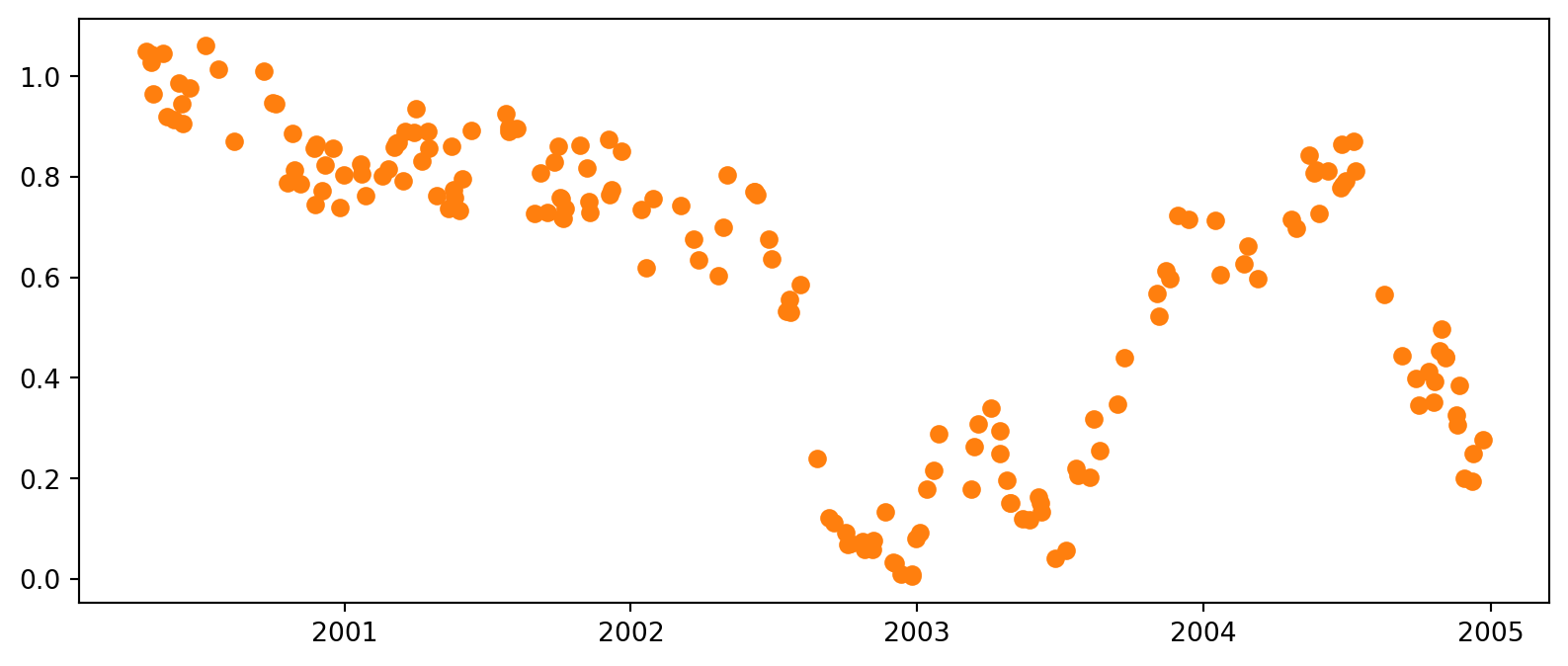
1.2. Proxy variable

In real-world scenarios, proxy variables can be obtained from various sources, such as:

Branded Search Volume: The volume of searches for the brand name on search engines.
Survey Data: Periodic surveys measuring brand recognition and recall among the target audience.
Social Media Engagement: Metrics such as likes, shares, comments, and mentions related

We simulate a proxy variable correlated with the true latent awareness effect, adding some noise to it.

import numpy as np

rng = np.random.default_rng(42)

proxy_variable = (
    true_effect[["latent/awareness"]] / true_effect["latent/awareness"].max()
)
proxy_variable *= rng.uniform(0.9, 1.1, size=len(proxy_variable)).reshape((-1, 1))

proxy_variable = proxy_variable.sample(n=180, random_state=42)

fig, ax = plt.subplots(figsize=(10, 4))
ax.scatter(
    proxy_variable.index.to_timestamp(),
    proxy_variable["latent/awareness"].values,
    color="C1",
    label="Proxy Variable",
)

2. Defining and Fitting the Model

We define a model that includes:

Piecewise linear trend
Yearly and weekly seasonality
Latent awareness, modeled a saturation function applied to the ad spend.
Awareness-to-sales effect, an effect that accounts the carryover aspect of awareness impact on sales.
Latent baseline, modeled as the sum of trend, seasonality, and awareness-to-sales effect
Last-click spend effect, modeled as a Hill saturation function multiplied by the latent baseline

The diagram below illustrates the model structure, including the latent variables and the proxy variable.

graph TD
    %% STYLES
    classDef latent fill:#dbeafe,stroke:#3b82f6,stroke-width:1px;
    classDef observed fill:#fef3c7,stroke:#f59e0b,stroke-width:1px;
    classDef proxy fill:#dcfce7,stroke:#16a34a,stroke-width:1px;
    classDef effect fill:#f3e8ff,stroke:#a855f7,stroke-width:1px;

    %% OBSERVED INPUTS
    X1["Ad Spend Awareness"]:::observed
    LastClick["Last-Click Spend"]:::observed
    Sales["Sales (y)"]:::observed

    %% LATENT STRUCTURE
    A_spend["Latent Ad Spend Awareness"]:::latent
    A_sum["Latent Awareness"]:::latent
    A_adstock["Latent Awareness Adstock"]:::latent
    Baseline["Latent Baseline (trend + seasonality + awareness)"]:::latent
    AwarenessToSales["Awareness → Sales Effect"]:::effect

    %% PROXY
    Proxy["Proxy Variable (e.g., Branded Search / Survey)"]:::proxy

    %% RELATIONSHIPS
    X1 -- "Hill saturation function (nonlinear spend response)" --> A_spend

    A_spend -- "Summed contribution" --> A_sum
    

    A_sum -- "Weibull adstock (carryover decay)" --> A_adstock
    A_adstock -- "Modulates baseline & seasonality" --> Baseline
    A_adstock -- "Drives multiplicative Awareness→Sales effect" --> AwarenessToSales

    AwarenessToSales -- "Direct causal effect on sales" --> Sales

    Baseline -- "Combines with last-click spend" --> LastClick
    LastClick -- "Final multiplicative effect on sales" --> Sales

    A_sum -- "Proportional proxy (γ·A + noise)" --> Proxy

    %% GROUPS
    subgraph Observed
        X1
        LastClick
        Sales
        Proxy
    end

    subgraph Latent_Model
        A_spend
        A_sum
        A_adstock
        Baseline
        AwarenessToSales
    end

We model the last-click effect as proportional to the latent brand awareness variable, which is influenced by upper-funnel marketing activities:

\[ \text{Hill}(X_{lc}(t)) \cdot \text{Baseline}(t) \]

where \(\text{Baseline}(t)\) includes the latent brand awareness effect, trend, and seasonality components. We basically assume that the last-click effect is stronger when brand awareness is higher, which is a reasonable assumption in many marketing contexts.

2.1. Model without Proxy Variable

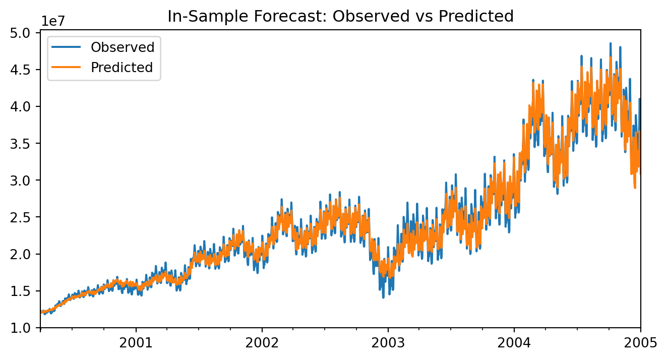
We first fit a baseline model without the proxy variable to see how it performs. Since last-click is highly correlated with sales, we will see how it overfits to last-click, leading to poor estimation of other components.

The cell below defines some effects (click to expand):

Code

from prophetverse.effects import (
    PiecewiseLinearTrend,
    LinearFourierSeasonality,
    ChainedEffects,
    GeometricAdstockEffect,
    WeibullAdstockEffect,
    HillEffect,
    SumEffects,
    Forward,
    Constant,
    MultiplyEffects,
)
from prophetverse.sktime import Prophetverse
from prophetverse.engine import MAPInferenceEngine
from prophetverse.engine.optimizer import LBFGSSolver
import numpyro.distributions as dist


# --- Defining seasonality and trend effects ---

trend = PiecewiseLinearTrend(changepoint_interval=300)

yearly = (
    "yearly_seasonality",
    LinearFourierSeasonality(
        freq="D",
        sp_list=[365.25],
        fourier_terms_list=[5],
        prior_scale=0.1,
        effect_mode="multiplicative",
    ),
    None,
)

weekly = (
    "weekly_seasonality",
    LinearFourierSeasonality(
        freq="D",
        sp_list=[7],
        fourier_terms_list=[3],
        prior_scale=0.05,
        effect_mode="multiplicative",
    ),
    None,
)


# --- Defining marketing effects ---

# First, we set up a Hill saturation object to be reused
hill = HillEffect(
    half_max_prior=dist.HalfNormal(1),
    slope_prior=dist.InverseGamma(2, 1),
    max_effect_prior=dist.HalfNormal(0.5),
    effect_mode="additive",
    input_scale=1e6,
)


# The effect of ad spend on awareness is modeled with a Hill function
# (nonlinear spend response)
spend_awareness = (
    "latent/awareness",
    hill,
    "ad_spend_awareness",
)


# The awareness does not impact sales immediately, but rather has a carryover effect. We model this with a Weibull adstock.
awareness_to_sales = (
    "awareness_to_sales",
    ChainedEffects(
        [
            ("saturation", Forward("latent/awareness")),
            ("adstock", WeibullAdstockEffect(max_lag=90)),
        ]
    ),
    None,
)

# The baseline is finally modeled as the sum of trend, seasonality, and latent awareness (considering adstock)
latent_baseline = (
    "latent/baseline",
    SumEffects(
        effects=[
            ("trend", Forward("trend")),
            ("yearly_seasonality", Forward("yearly_seasonality")),
            ("weekly_seasonality", Forward("weekly_seasonality")),
            ("awareness", Forward("awareness_to_sales")),
        ]
    ),
    None,
)


chained_last_click = (
    "last_click_spend",
    MultiplyEffects(effects=[("hill", hill), 
    ("baseline", Forward("latent/baseline"))]),
    "last_click_spend",
)

baseline_model = Prophetverse(
    trend=trend,
    exogenous_effects=[
        yearly,
        weekly,
        spend_awareness,
        awareness_to_sales,
        latent_baseline,
        chained_last_click,
    ],
    inference_engine=MAPInferenceEngine(
        num_steps=5000,
        optimizer=LBFGSSolver(memory_size=300, max_linesearch_steps=300),
    ),
)
baseline_model.fit(y=y, X=X)

Let’s visualize the predictions of this baseline model:

y_pred = baseline_model.predict(X=X, fh=X.index)

plt.figure(figsize=(8, 4))
y.plot(label="Observed")
y_pred.plot(label="Predicted")
plt.title("In-Sample Forecast: Observed vs Predicted")
plt.legend()
plt.show()

Forecast quality alone does not tell the full story of how well the model is capturing the underlying dynamics.

Component-Level Diagnostics

With predict_components, we can obtain the model’s components.

y_pred_components_baseline = baseline_model.predict_components(X=X, fh=X.index)

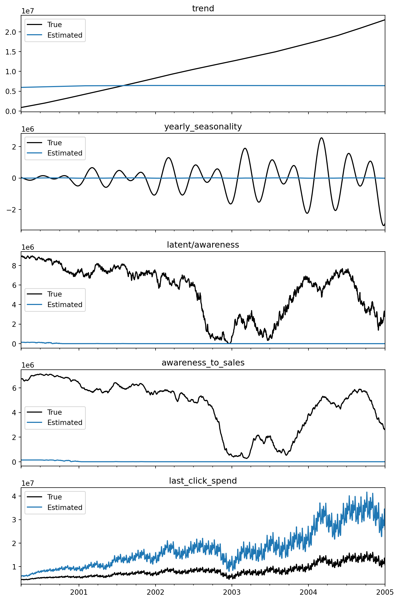
Since we have access to the ground truth of the components in this synthetic example, we can compare them to see how well the model is capturing the true effects.

fig, axs = plt.subplots(5, 1, figsize=(8, 12), sharex=True)
for i, name in enumerate(
    [
        "trend",
        "yearly_seasonality",
        "latent/awareness",
        "awareness_to_sales",
        "last_click_spend",
    ]
):
    true_effect[name].plot(ax=axs[i], label="True", color="black")
    y_pred_components_baseline[name].plot(ax=axs[i], label="Estimated")
    axs[i].set_title(name)
    axs[i].legend()
plt.tight_layout()
plt.show()

Since the last-click spend is highly correlated with sales, the model tends to over-attribute sales to the last-click effect, leading to poor estimation of other components, especially the latent awareness effect.

2.2. Model with Proxy Variable

We use LinearProxyLikelihood to add the proxy variable to the model. This effect links the latent awareness variable to the observed proxy variable, helping to better identify the latent effect.

Since we know that the correlation is positive, we use a HalfNormal prior for the coefficient.

from prophetverse.effects.proxy_likelihood import LinearProxyLikelihood


proxy_effect = (
    "awareness_proxy",
    LinearProxyLikelihood(
        effect_name="latent/awareness",
        reference_df=proxy_variable,
        coefficient_prior=dist.HalfNormal(0.2),
        likelihood_scale=0.05,
    ),
    None,
)

model = Prophetverse(
    trend=PiecewiseLinearTrend(changepoint_interval=300),
    exogenous_effects=[
        yearly,
        weekly,
        spend_awareness,
        awareness_to_sales,
        latent_baseline,
        chained_last_click,
        proxy_effect,
    ],
    inference_engine=MAPInferenceEngine(
        num_steps=5000,
        optimizer=LBFGSSolver(memory_size=300, max_linesearch_steps=300),
    ),
)

model.fit(y=y, X=X)

Let’s visualize the predictions of this proxy variable model:

y_pred_model = model.predict(X=X, fh=X.index)

plt.figure(figsize=(8, 4))
y.plot(label="Observed")
y_pred_model.plot(label="Predicted")
plt.title("In-Sample Forecast: Observed vs Predicted")
plt.legend()
plt.show()

Component-Level Diagnostics

With predict_components, we can obtain the model’s components.

y_pred_components = model.predict_components(X=X, fh=X.index)

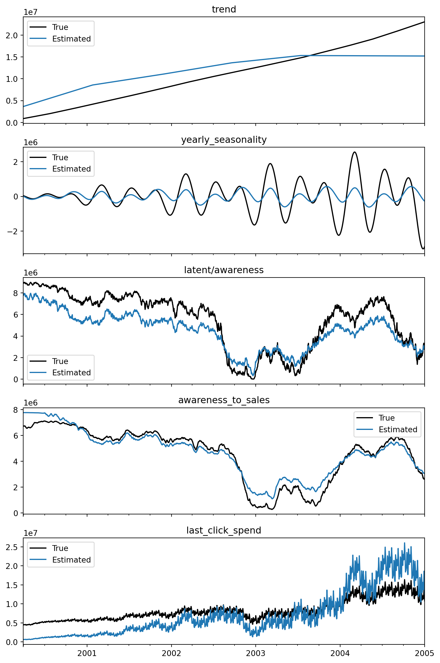
In a real use-casee, you would not have access to the ground truth of the components. We use them here to show how the model behaves, and how incorporing extra information can improve it.

fig, axs = plt.subplots(5, 1, figsize=(8, 12), sharex=True)
for i, name in enumerate(
    [
        "trend",
        "yearly_seasonality",
        "latent/awareness",
        "awareness_to_sales",
        "last_click_spend",
    ]
):

    true_effect[name].plot(ax=axs[i], label="True", color="black")
    y_pred_components[name].plot(ax=axs[i], label="Estimated")
    axs[i].set_title(name)
    axs[i].legend()
plt.tight_layout()
plt.show()

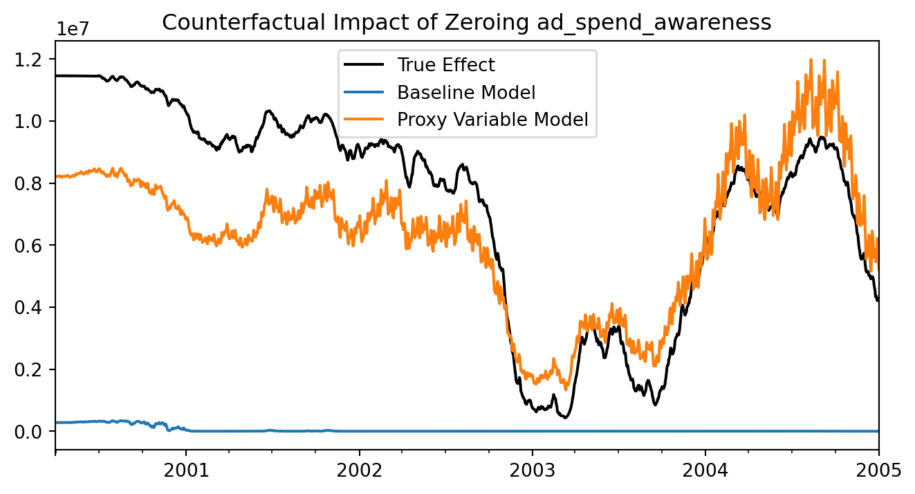
3. Comparing models

Here, we do our final comparison of the models, looking at the counterfactual impact of zeroing out the awareness ad spend. This shows how important it is to include the proxy variable to correctly attribute the impact of awareness spend.

def plot_compare_models(column):

    delta_true = get_counterfactual(true_model, X, column)
    delta_baseline = get_counterfactual(baseline_model, X, column)
    delta_proxy = get_counterfactual(model, X, column)

    plt.figure(figsize=(8, 4))
    delta_true.plot(label="True Effect", color="black")
    delta_baseline.plot(label="Baseline Model")
    delta_proxy.plot(label="Proxy Variable Model")
    plt.title(f"Counterfactual Impact of Zeroing {column}")
    plt.legend()
    plt.show()


plot_compare_models("ad_spend_awareness")

We see that, although not perfect, the model with the proxy variable is able to much better capture the true impact of awareness spend on sales, while the baseline model without the proxy variable fails to do so.

How to cite this package

If you use Prophetverse or any of this idea in your package/paper, please cite this package according to DOI on Readme.