Prophetverse

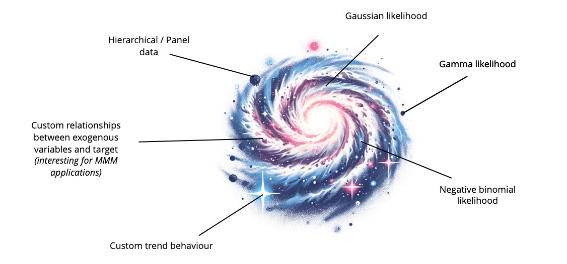
Figure 1: Generalized Additive Models are versatile. Prophet is one of the many models that can be built on top of it. The idea of Prophetverse is giving access to that universe.

Prophetverse leverages the Generalized Additive Model (GAM) idea in the original Prophet model and extends it to be more flexible and customizable. The core principle of GAMs is to model the expected value \(y_{mean}\) of the endogenous variable \(Y\) as the sum of many functions \(\{f_i\}_{i=1}^n\) of exogenous variables \(\{x_i\}_{i=1}^n\).

\[ y_{mean} = f_1(x_1) + f_2(x_2) + \ldots + f_n(t)\text{, }\quad n \in \mathbb{N} \]

The innovation in Prophet is the use of Bayesian GAMs to model time series data. Instead of approximating the time series through auto-regressive models, Prophet treats it as a curve-fitting exercise. This approach results in fast, interpretable, and accurate forecasts. The Prophet formulation is:

\[ y_{\text{mean}} = \begin{cases} y_{\text{mean}}(t) = \tau(t) + s(t) + h(t) + v(t) & \text{if additive} \\ y_{\text{mean}}(t) = \tau(t) + \tau(t) \cdot s(t) + \tau(t) \cdot h(t) + \tau(t) \cdot v(t) & \text{if multiplicative} \end{cases} \]

where \(\tau(t)\) is the trend component, \(s(t)\) is the seasonality component, \(h(t)\) is the holiday component, and \(v(t)\) is other regressors components. Those components are hard-coded as linear in the original formulation of Prophet, but in Prophetverse they are versatile and can be defined by the user. This is the first main difference between Prophet and Prophetverse. The \(f_i\) functions are defined by the Effects API, where the user can create their own components and priors, by using the already available ones or by creating new BaseEffect subclasses.

\[\begin{align} y_{mean} &= \sum\limits_{i=1}^n f_i(x_i(t), \{f_j(x_j)\}_{j<i}) \\ &= f_1(x_1(t)) + f_2(x_2(t), f_1(x_1(t))) + \ldots + f_n(t, \{f_j(x_j)\}_{j<n}) \end{align}\]

where \(f_1\), the first component, accounts for the trend. This definition superseeds the Prophet formulation. Effects are ordered, so that the output of previous effects can be used as input for the next ones. This allows for complex interactions between exogenous variables.

Likelihood

In the original Prophet, the likelihood is a Normal distribution, but in Prophetverse it can be Normal, Gamma, or Negative Binomial.

\[ y \sim \mathcal{likelihood}(\phi(\hat{y}_{mean}), \sigma^2)\quad \text{where} \quad \sigma \sim HalfNormal(\sigma_{hyper}) \]

where \(\sigma_{hyper}\) is a hyperparameter and \(\phi\) is a function that maps the mean to the support of the likelihood. For normal likelihood, \(\phi\) is the identity function, but for Gamma and Negative Binomial, it is

\[ \phi(k) = \begin{cases} k & \text{if } k > 10^5 \\ z\exp(k-z) & \text{if } k \leq z \end{cases} \]

for some small threshold \(z\). We set \(z = 10^{-5}\) in our implementation. The reason for this is to avoid zero or negative values in the support of the likelihood, which can lead to error.

Trend

There are mainly two types of trends supported: linear and logistic. We will first take a look at the original mathematical formulation of Prophet's paper, and then simplify it to obtain a simpler and more interpretable version.

Linear trend

Original formulation

The linear trend is modeled as a piecewise linear functions with changepoints. Let \(M\) be the number of changepoints, \(\delta \in \mathbb{R}^M\) be the rate adjustment at each changepoint, \(\{\kappa_i\}_{i=1}^M\) be the changepoint times, and be \(a(t) \in \{0,1\}^M\) be a vector which assumes, at each index, 1 if the corresponding changepoint is greater than \(t\) and 0 otherwise. In addition, let \(k\) represent the global rate and \(m\) the global offset. Then, the linear trend is defined as:

\[ \tau(t) = (k + a(t)^T\delta)t + (m + a(t)^T\gamma), \quad \text{where} \quad \gamma_i = \kappa_i\delta_i \]

The first part accounts for the rate adjustment at each changepoint, and the second part corrects the offset at each changepoint, so that the trend is continuous.

Prophetverse's equivalent formulation

This can be simplified as a first-order spline regression with \(M\) knots (changepoints). Let \(b(t) \in \mathbb{R}^M\) be a vector so that \(b(t)_i = (t - \kappa_i)_+\) (the positive part of \(t - \kappa_i\)). Then, the piecewise linear trend value for time \(t\) can be written as:

\[ \tau(t) = b(t)^T \delta + kt + m \]

We can also write the trend for all \(t \in \{t_1,\dots, t_T\}\) as a matrix multiplication. Let \(\mathbf{B} \in \mathbb{R}^{T \times M+2}\) be the matrix whose rows are \(b'(t) = \left[ b(t), t, 1 \right]\) for each time \(t\). In other words, it is the spline basis matrix. The \(t\) and \(1\) at the end of the vector are included to account for the global rate and offset. Furthermore, consider the vector \(\delta' = \left[ \delta, k, m \right]\). Then, the trend vector \(G \in \mathbb{R}^T\), \(G_i = \tau(\mathbf{t}_i)\), can be written as:

\[\begin{align} G &= \mathbf{B}\delta' \\ \end{align}\]

\[\begin{align} G &= \begin{bmatrix} (t_0 - \kappa_0)_+ & (t_0 - \kappa_1)_+ & \ldots & (t_0 - \kappa_{M-1})_+ & t_0 & 1 \\ (t_1 - \kappa_0)_+ & (t_1 - \kappa_1)_+ & \ldots & (t_1 - \kappa_{M-1})_+ & t_1 & 1 \\ \vdots & \vdots & \ddots & \vdots & \vdots & \vdots \\ (t_{T-1} - \kappa_0)_+ & (t_{T-1} - \kappa_1)_+ & \ldots & (t_{T-1} - \kappa_{M-1})_+ & t_{T-1} & 1 \\ \end{bmatrix} \begin{bmatrix} \delta_0 \\ \delta_1 \\ \vdots \\ \delta_{M-1} \\ k \\ m \\ \end{bmatrix} \end{align}\]

Example

One possible realization of \(\mathbf{B}\) is:

\[ \begin{bmatrix} 0 & 0 & 0 & 0 & 0 & 1 \\ 0 & 0 & 0 & 0 & 1 & 1 \\ 1 & 0 & 0 & 0 & 2 & 1 \\ 2 & 1 & 0 & 0 & 3 & 1 \\ \vdots & \vdots & \vdots & \vdots & \vdots & \vdots \\ T-1 & T-2 & T-3 & T-4 & T-1 & 1 \\ \end{bmatrix} \]

Logistic trend

The logistic trend of the original model uses the piecewise logistic linear trend to change the rate at which \(t\) grows. We will not explain the mathematical formulation of the original paper here, and will already leverage what we have learned about the linear trend to simplify it.

\[ G = \frac{C}{1 + \exp(-\mathbf{B}\delta')} \]

where \(C\) is the logistic capacity, which should be passed as input to Prophet, but is a random variable in Prophetverse.

Changepoint priors

A Laplace prior is put on the rate adjustment \(\delta_i \sim Laplace(0, \sigma_{\delta})\) where \(\sigma_{\delta}\) is a hyperparameter. The changepoint times \(\kappa_i\) can be predefined by the user, or can be uniformly distributed in the training data. The offset and rate prior location are set in a "smart" way, by checking analytically what would be the values that fit the maximum and minimum points of the time series.

Note

Although those trend are the ones that come with the library, the user can define any trend, including a trend that depends on some exogenous variable. Flexibility is the key here.

Seasonality

To model seasonality, Prophet uses a Fourier series to approximate periodic functions, allowing the model to fit complex seasonal patterns flexibly. This approach involves determining the number of Fourier terms (K), which corresponds to the complexity of the seasonality. The formula for a seasonal component s(t) in terms of a Fourier series is given as:

\[ s(t) = \sum_{k=1}^K \left( a_k \cos\left(\frac{2\pi kt}{P}\right) + b_k \sin\left(\frac{2\pi kt}{P}\right) \right) \]

Here, P is the period (e.g., 365.25 for yearly seasonality), and \(a_k\) and \(b_k\) are the Fourier coefficients that the model estimates. The choice of K depends on the granularity of the seasonal changes one wishes to capture. A Normal prior is placed on the coefficients, \(a_k, b_k \sim \mathcal{N}(0, \sigma_s)\), where \(\sigma_s\) is a hyperparameter.

Matrix Formulation of Fourier Series

To efficiently compute the seasonality for multiple time points, we can represent the Fourier series in a matrix form. This method is especially useful for handling large datasets and simplifies the implementation of the model in computational software. Let \(T\) be the number of time points, and create a design matrix \(X\) of size \(T \times 2K\). Each row of \(X\) corresponds to a time point and contains all Fourier basis functions evaluated at that time:

\[ \mathbf{X} = \begin{bmatrix} \cos\left(\frac{2\pi \cdot 1 \cdot t_1}{P}\right) & \sin\left(\frac{2\pi \cdot 1 \cdot t_1}{P}\right) & \cdots & \cos\left(\frac{2\pi \cdot K \cdot t_1}{P}\right) & \sin\left(\frac{2\pi \cdot K \cdot t_1}{P}\right) \\ \cos\left(\frac{2\pi \cdot 1 \cdot t_2}{P}\right) & \sin\left(\frac{2\pi \cdot 1 \cdot t_2}{P}\right) & \cdots & \cos\left(\frac{2\pi \cdot K \cdot t_2}{P}\right) & \sin\left(\frac{2\pi \cdot K \cdot t_2}{P}\right) \\ \vdots & \vdots & \ddots & \vdots & \vdots \\ \cos\left(\frac{2\pi \cdot 1 \cdot t_T}{P}\right) & \sin\left(\frac{2\pi \cdot 1 \cdot t_T}{P}\right) & \cdots & \cos\left(\frac{2\pi \cdot K \cdot t_T}{P}\right) & \sin\left(\frac{2\pi \cdot K \cdot t_T}{P}\right) \end{bmatrix} \]

Coefficient Vector:

Define a vector \(\beta\) of length 2K containing the coefficients \(a_1, b_1, \dots, a_K, b_K\):

\[ \mathbf{\beta} = \begin{bmatrix} a_1 \\ b_1 \\ \vdots \\ a_K \\ b_K \end{bmatrix} \]

The seasonality for all time points can then be computed through the matrix product of \(X\) and \(\beta\):

\[ \mathbf{s} = \mathbf{X} \mathbf{\beta} \]

Each element of vector \(s\), denoted as \(s_i\), represents the seasonality at time \(t_i\).

This matrix approach not only makes the computation faster and more scalable but also simplifies integration with other components of the forecasting model. One drawback is that it assumes a constant seasonality, but an user can also define a seasonality that changes with time in Prophetverse, by creating a custom Effect class.

Multivariate model

Prophetverse also supports multivariate forecasting. In this case, the model is essentially the same, but for now only Normal Likelihood is supported. Depending on the usage of the library, we may add other likelihoods in the future (please open an issue if you need it!). In that case, all other components are estimated in the same way, but the likelihood is a multivariate distribution. The mean of the distribution is a vector, and the covariance matrix prior is a LKJ distribution.